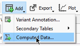
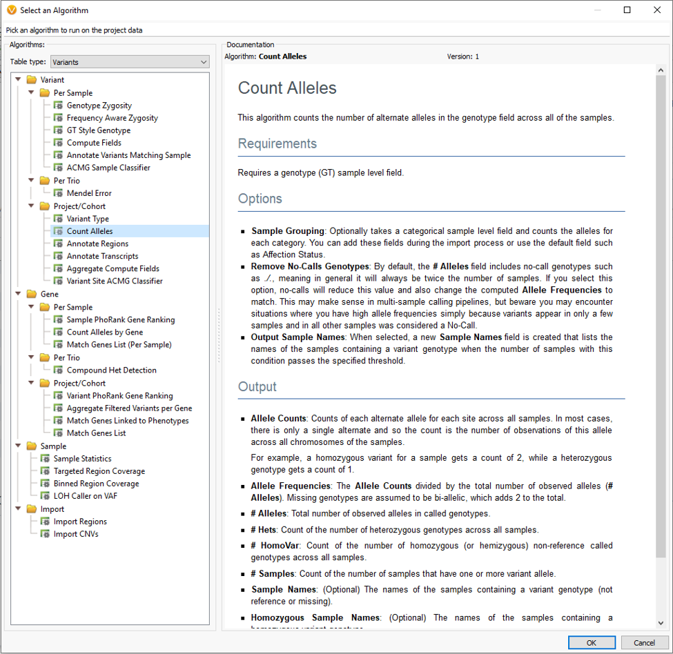
Although VarSeq is intentionally designed to be a clinical NGS pipeline tool able to run a handful or even single samples through, we have many users who run large cohort style studies with the tool as well. One common use is to compare case/control data to isolate variants shared among affected individuals and exclude those in unaffected. One incredibly powerful tool to use for this and many other analyses is the Count Alleles Algorithm (Fig 2). You’ll find this tool listed under Computed Data (Fig 1).
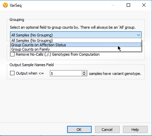
Each algorithm comes with a general application description, list of required fields and expected output. The Count Alleles Algorithm can be run in a number of ways. Some simple approaches are to count the variants across all samples in a project, break variant counts down by affection status, or additionally add unique sample groups like location or family name (Fig 3).
The output is a number of fields meant to clarify how shared variants are distributed among the samples in the project. Each of these fields can be added to the filter chain to prioritize variants of high/low frequency, any that are heterozygous or homozygous states, sample names, and in this specific case any present among affected/unaffected samples.
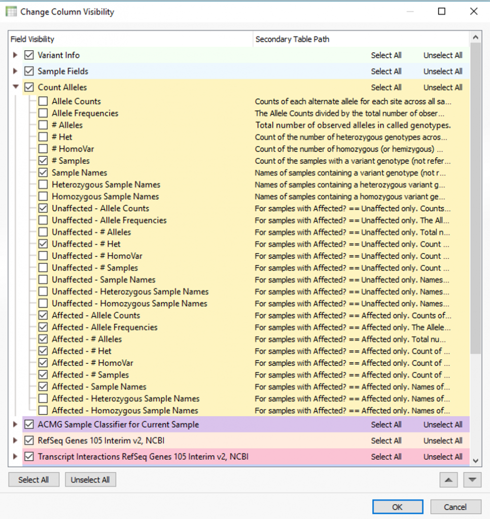
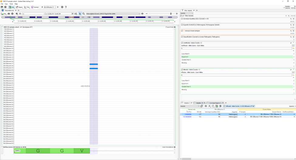
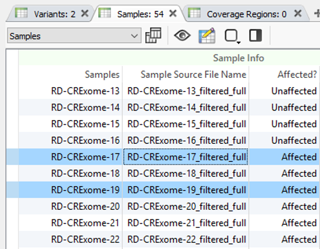
Using two of the fields in Fig. 4 as filters, Fig. 5 shows the results of finding high-quality variants (GQ >= 50), in heterozygous or homozygous state, removing known benigns in ClinVar, Likely pathogenic or pathogenic variants from the ACMG Classifier, and finally, the remaining variants not found in unaffected samples (allele counts = 0) and shared among affected individuals (allele counts > 0). The results show two variants shared among a few affected samples in the project. You can find the affection status labels in the samples table (Fig 6).
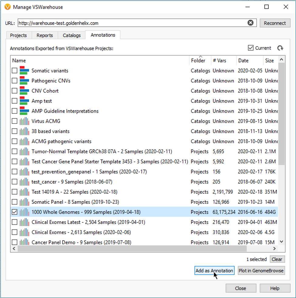
The Count Alleles Algorithm is also integral for uploading project data into VSWarehouse. Essentially, the allele counts, and frequencies are leveraged from Warehouse as filterable fields for taking mass cohort data across many projects and samples to prioritize variants with low allele frequencies. A good example here is to eliminate common variants that are either real or possible false positives, which easily scales to millions of variants (Fig 7).
This blog is meant to just highlight the value of our Count Alleles Algorithm. If you have any specific questions on application please reach out to info@goldenhelix.com and we can schedule a call to discuss how to implement the algorithm into your project.