In many cases, VarSeq users design their next-gen sequencing workflows for a clinical application. One of the major values of using VarSeq is the standardization of sample analysis via project templates for filtering down to rare variants and isolate any clinically relevant variant. However, VarSeq also doubles as a robust research application as well. There are specific algorithms that can be beneficial to a research project, but the biggest consideration for workflow is focused on the filtering strategies. The purpose of this blog is to expose readers to the nuances of filtering and other tools in VarSeq that may prove useful for any cohort analysis. We’ll start things by looking at a typical clinical workflow to break down filtering strategies as we look at VarSeq NGS workflows for clinical and research.

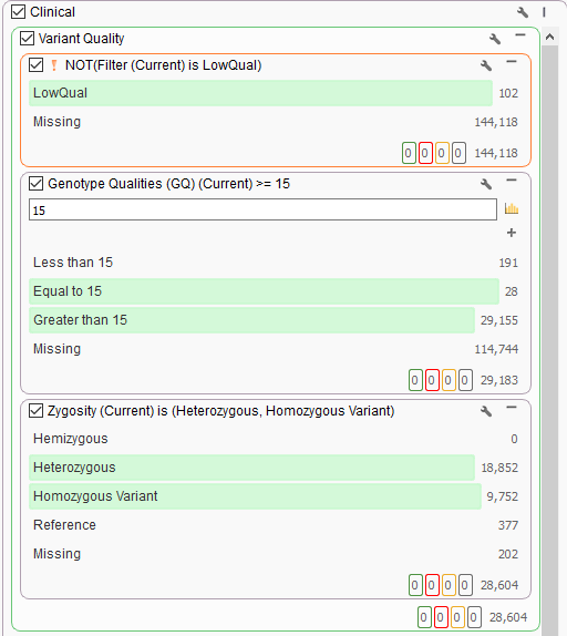
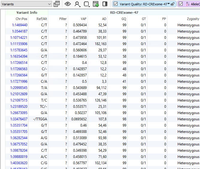
One advantage of VarSeq is that users can define their filtering strategy however they wish. In a clinical scenario, it is really common to utilize the variant quality fields as a first pass filtering strategy. These are the quality fields contained in the VCF and generated from the secondary analysis pipeline handling alignment and calling. Every field in the VCF will be imported into VarSeq and optional for filtering. For those well versed in VCF format, you are aware of the two types of fields in the file being the “Info” fields generic to the variant, and “Format” fields specific to the variant in a given sample. It is the “Format” fields that are used to focus on any high-quality variants present in the sample and therefore begins the clinical filtering focus on one sample at a time. Figures 1a and 1b show these fields in the filter chain and variant table. Common fields used in this case may be genotype quality scores, read depth, zygosity computed from the GT field, or calculated variant allele frequency from allelic depth values.

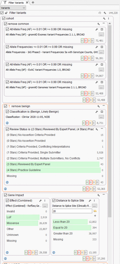
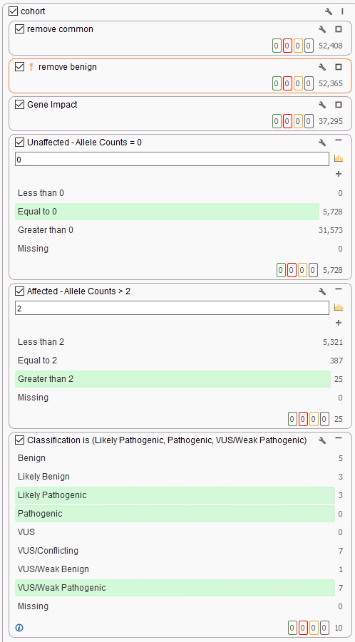
A typical strategy may be to only import one sample into a VarSeq project, but if the goal is to run batches, these sample level filters are crucial for the per-sample review. Alternatively, if the goal of the workflow is to isolate potentially interesting variants seen among a cohort, the filtering strategy has to be modified. Instead of isolating variants in a given sample, create a filter chain that works on generic variant level fields. A fantastic example is for allele frequency thresholds using population catalogs, much like gnomAD or 1000 Genomes. An example filter can be seen below where allele frequency thresholds are set to keep variants that occur at a rate of 1% or less among the population across multiple population frequency databases (i.e., gnomAD genomes and exomes, 1kG Phase3, and ExAC. Additionally, this filter includes criteria to remove well-known benign variants from ClinVar and focus on the loss of function, missense, and potential splicing variants utilizing RefSeq genes.

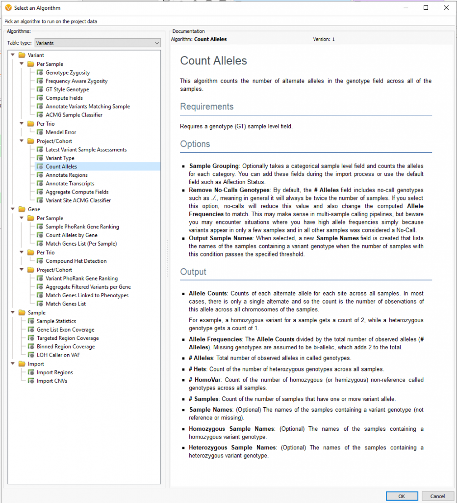
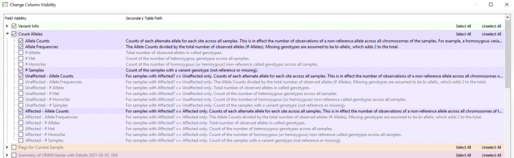
Moreover, users can implement the count alleles algorithm to assist in isolating variants seen commonly among affected individuals while removing variants present in unaffected samples. This algorithm (Figure 3a and 3b) is beneficial in not only finding unique variants across affected samples but can also be used to eliminate common variants among the whole cohort, otherwise likely artifacts.

This tool can then be added to the previous cohort filter to remove variants in unaffected samples (Unaffected – Allele Counts = 0) and keep any variants present in affected samples (Affected – Allele Counts > 2). This was paired with the prioritization of potentially pathogenic variants using the ACMG variant site classifier (Figure 4).

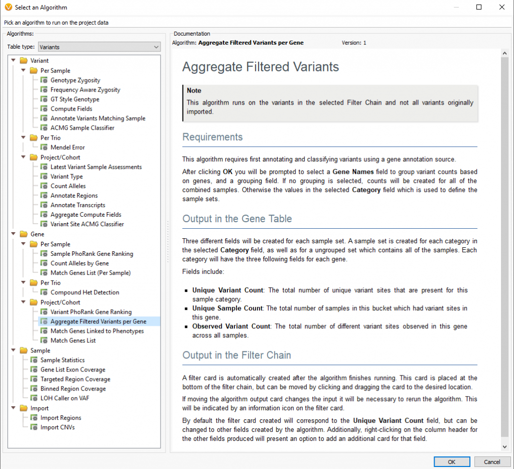
Another helpful algorithm is the Aggregate Filtered Variants Per Gene (Figure 5). The workflow above is great for finding the same variant across multiple samples. Still, you also need the option to aggregate any potential variants of interest across the gene level for all affected samples. This is one of the few algorithms that work off of the current status of the filter chain. Meaning it will only aggregate the filtered variants from the resulting workflow above.

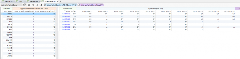
This is best displayed in an alternative table layout showing Variants by Variant Genes. Meaning, you can quickly browse the total number of filtered variants distributed across each gene for the affected samples at the bottom of your filter. You’ll see the gene list sorted for the highest number of unique variant counts for the affected samples in Figure 6. In other words, what are my potential candidate genes for the affected samples even if each affected sample has independent variants in that gene.

Obviously, each research project is going to have nuanced strategies for isolating these interesting variants. This blog aims to expose our users to these advanced tools that may not get utilized as commonly as some of the other clinically focused algorithms. I encourage our users to explore these features, become familiar with their utilization, and determine if they could add value to any potential cohort project. The main workflow differentiator will be the filtering strategy, where, if in a clinical application, rely on sample level fields like those provided in the VCF format fields. However, if wishing to explore variants in a cohort, stick to using generic variant level fields. I hope this adds some clarity to building your projects, but please do not hesitate to reach to info@goldenhelix.com if you would like more formal training. If you enjoyed this content, please check out some of our other blog posts, which contain important information and updates on our clinical interpretation capabilities.