
Unlock the potential of VarSeq for efficient analysis of structural variants, providing robust annotation, filtering, and interpretation of intricate genetic variations.
While the analysis of structural variants (SVs) is crucial for understanding the genetic basis of disease, the process of interpreting these variations can be a challenging and complex task. Structural variant callers typically store rearrangements in VCF files, which are encoded using a complex breakend notation. While this notation is capable of describing the full spectrum of structural variation, it does not capture all of the information necessary to interpret a given SV. Fortunately, VarSeq provides a robust set of features for the annotation, filtering, and interpretation of SVs.
This blog post will explore the creation of a tertiary analysis workflow for the interpretation of SVs using VarSeq. To illustrate this process, we will use hypothetical whole-exome sequencing data from a patient diagnosed with severe combined immunodeficiencies.
Importing Structural Variants
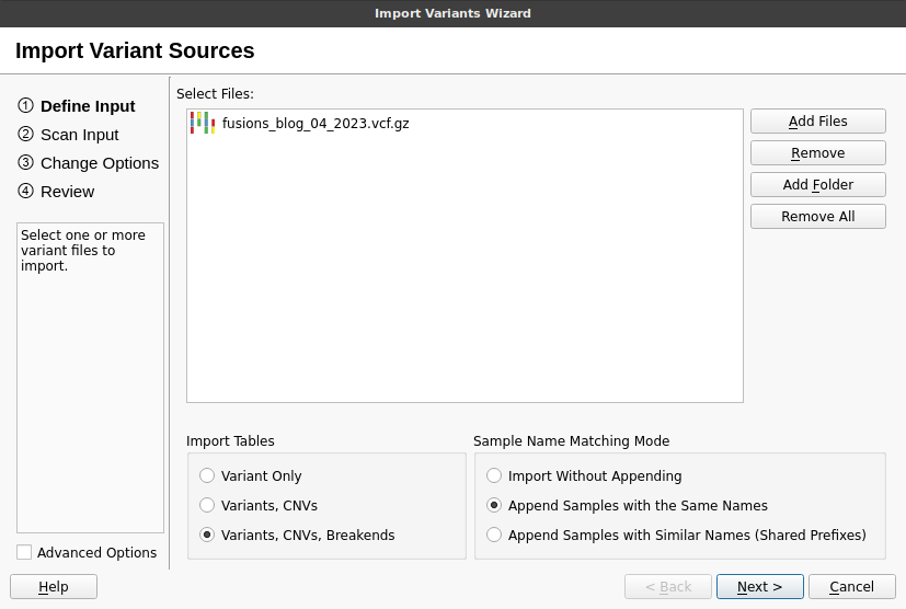
We will begin by importing the VCF file for our patient into an empty VarSeq project. VarSeq supports the analysis of all classes of genomic variation in a sample and allows the import of small variants, copy number variants (CNVs), and SVs from a single VCF file. To begin the import process, click Import Variants, then click Add Files and select the VCFs containing the SVs for the sample. Next, click the Variants, CNVs, and Breakends radio button to import all three types of variation. Finally, click Next and follow the instructions in the wizard to complete the import process.
During the import process, VarSeq automatically joins breakend mate pairs and infers the type of each SV on import. Once the import is complete, three tables are created for each type of variation:
- Variants
- CNVs
- Breakends
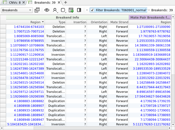
Any CNVs that are described using breakend notation are imported into both the Breakend and CNV tables so that they can be annotated and interpreted in either context. The Breakend table provides several useful fields for the interpretation of structural variants, including the Type, Orientation, and Mate Strand.
Annotation and Filtering
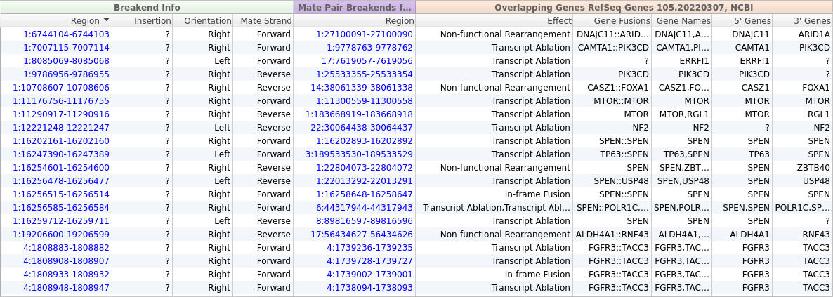
From the screenshot above, we can see that we have imported 39 SVs, but most of these variants will not be relevant to our patient’s phenotype. Fortunately, we can use VarSeq’s powerful annotation and filtering capabilities to identify a small set of clinically relevant SVs. We will start by adding gene annotations to our Breakend table by clicking Add -> Secondary Tables -> Breakend Annotation and then selecting for RefSeq Genes in the annotation dialog. The gene annotation algorithm provides us with details about any gene fusions produced by a given SV, along with an Effect field describing the predicted effect of the SV on the protein product.
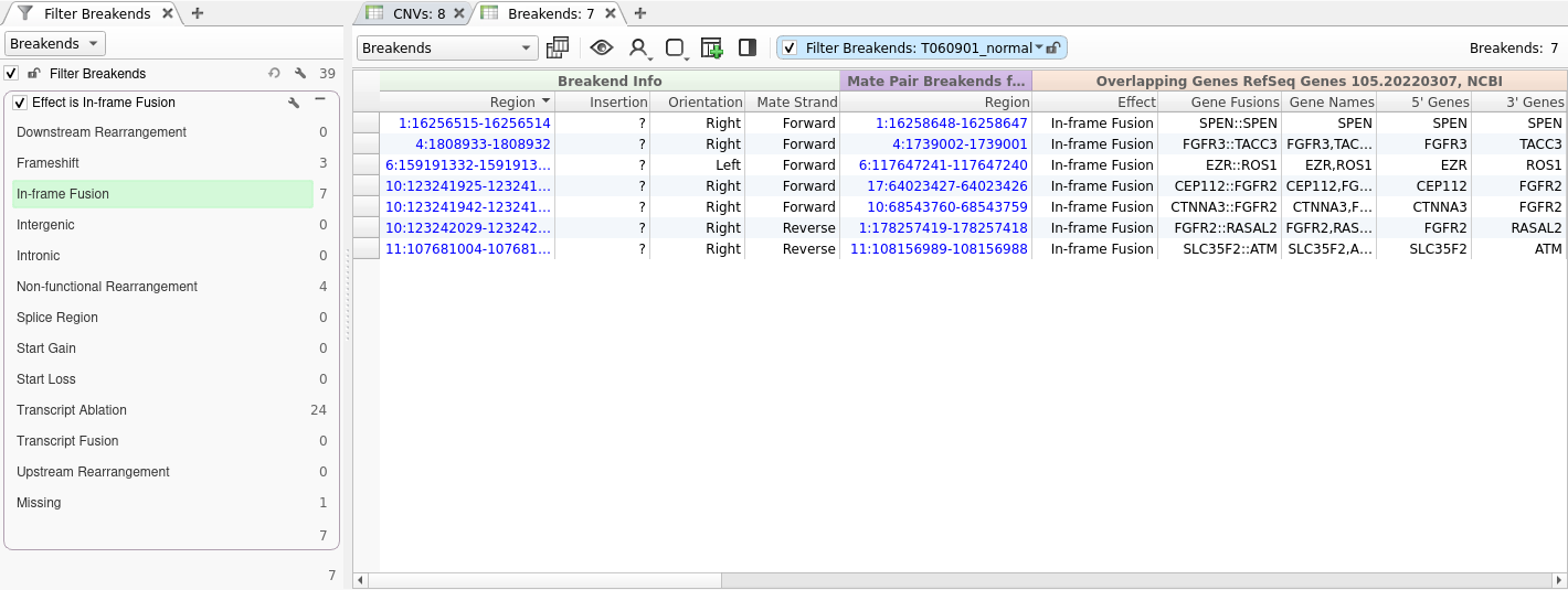
Now that we have performed gene annotation, we can filter down to the set of SVs that are predicted to result in an in-frame protein fusion by right-clicking on the Effect field and selecting Add to Filter Chain. Next, we will select In-frame Fusion from the list of effects. This gets us down to a list of just seven SVs.
After filtering on effect, we will create a gene panel filter to identify SVs in genes associated with our patient’s phenotype. This is a new feature that will be supported in the upcoming VarSeq release this spring. For this example, we will be using the Primary Immunodeficiency gene panel from the Panel App knowledgebase. This panel can be added from the Tools -> Manage Gene Panels dialog.
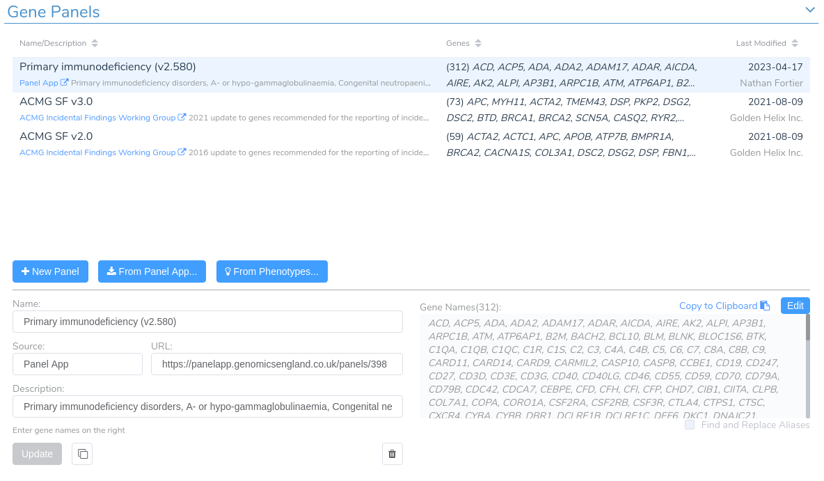
We can add a gene panel filter by right-clicking the filter chain and selecting Add Gene Panel Filter. Next, we select the Gene IDs field and click OK. In the newly added gene panel filter, we will select the Primary Immunodeficiency panel from the drop-down.

After adding this filter, we are left with a single SV that can now be interpreted and added to a clinical report in VSClinical.
Conclusion
This blog post demonstrated how VarSeq’s powerful filtering and annotation capabilities can be leveraged to create a tertiary analysis workflow for the interpretation of SVs. VarSeq greatly simplifies the SV interpretation process by automatically determining the type of each SV and predicting each variant’s effect on the resulting protein product. After performing annotation, SVs can be filtered down to a set of events that are relevant to the patient’s phenotype. If you have any questions about structural variant support in VarSeq, please don’t hesitate to contact us at support@goldenhelix.com.