As our final part of the ‘Top-Quality GWAS Analysis’ blog series, we will be giving a summary of the values behind GWAS quality control and quality assessment. Performing GWAS can provide insight into the association of genetic variants with traits and complex disorders. Any novel insights into marker-phenotype associations need to be based on performing quality control steps. In this blog series, we’ve explored many sample, marker, and population quality control methods. Following these quality control steps, we can then use the data to run clean association tests, which will be the focus of this blog.
As Darby illustrated previously, Principle Component Analysis (PCA) can be used to detect underlying population stratification. Population stratification or artifacts in allele frequencies between subpopulations in a population can confound association tests. Thus, the next step after performing PCA is to apply the results to a genotype association Test. This can be done under the Genotype > Genotype Association Tests dialog. In the dialog shown in figure 1, we will select to output data for P-P/Q-Q plots. But, we will also correct for stratification with PCA.
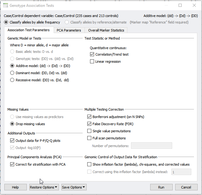
Fig 1: Performing Genotype Association Test and selecting to correct for stratification with PCA.
If you have not already performed PCA within your project, selecting to correct for stratification with PCA will perform this analysis from scratch. However, a precomputed PCA can also be applied using the PCA parameters tab at the top of the dialog in Figure 1 and 2. In the PCA parameters tab, select “Use precomputed principle components” and select your Principle Component sheet. The output will provide you with a new association test that accounts for population stratification as well as quality-filtered data.
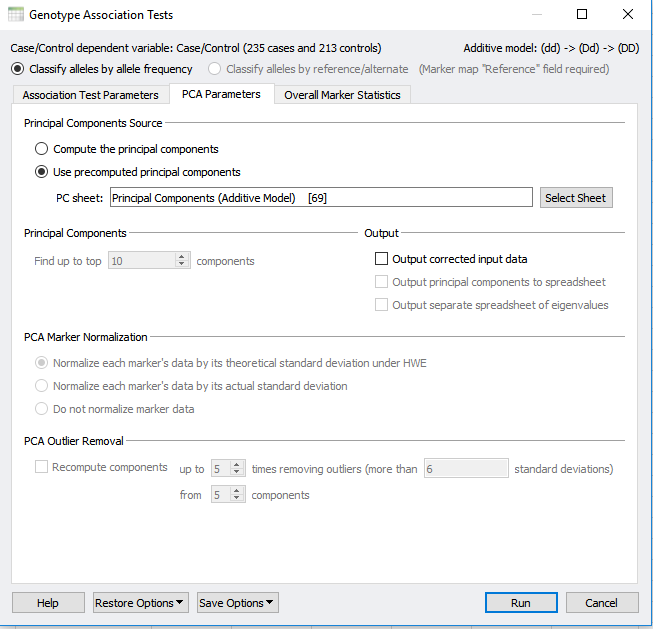
Fig 2: Under the PCA parameters tab you can select for a precomputed Principle Component sheet.
Potential Inflation of Significant Markers
The next step is to visualize potential inflation of significant markers output from the association test. The first plot that we can assess to determine quality assurance is the Q-Q plot. This plot is a scatter plot comparing the expected vs. observed -log10 P-values and will identify inflation in your data. As you can see in Figure 3, the expected vs. observed P-values correlate nicely with the slope, indicating that we have successfully removed bias in the data.
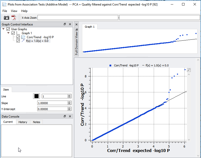
Fig 3: Q-Q plot is demonstrating quality assurance.
Visualizing the Data
The last step is visualizing the data in a Manhattan plot, which can be plotted using the Corr/Trend -log10 P-values in your Association Test result. For comparison, we plotted in Figure 4 an association test without (top) and with (bottom) data quality management. Notice the suppressed marker significance int the bottom plot, showing that the inflated p-values are prevented. Using this data, we can now identify SNPs that are associated with our observable trait and perform downstream analyses, such as imputation and genomic prediction.
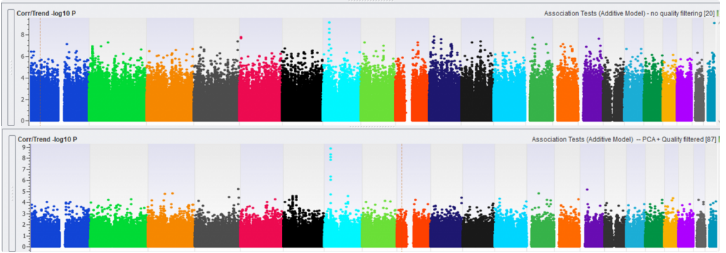
Fig 4: Manhattan plot without (top) and with (bottom) data quality management.
SVS is an ideal setup for GWAS analysis that can be applied to many different domains of life. Through this blog series, we have discussed assessing for sample and marker statistics, LD pruning, sample relatedness, and population stratification. All of these steps are important for data quality management. Additionally, they will help in identifying marker-phenotype associations and candidate gene targets for clinical and research application fields. Hopefully, you have enjoyed this blog series and can implement these steps into your practices. If you have any questions on these methods or other tools in SVS, please contact us at support@goldenhelix.com.