Sample Relatedness
Pruning your data based on Linkage Disequilibrium (LD) values and filtering for sample “relatedness” are ideal quality assurance steps following the marker and sample quality filtering described in Part II of this blog series. The value of running an Identity by Decent estimation not only allows you to factor family relatedness in your samples but makes screening for possible duplicate samples that may exist in your cohort. Any IBD test will perform better if you first prune markers so to eliminate linkage disequilibrium.
What is Linkage Disequilibrium?
Linkage Disequilibrium (LD) refers to the degree to which an allele of one SNP is inherited or correlated to the allele of another SNP (Bus & Moore, 2012). It is based on the concept that recombination events in a fixed population undergoing random mating will break apart chromosomal regions. The chromosomal regions that remain together, however, throughout the population are defined as chromosomal linkage or are in LD with each other. Because of this, LD is important to take into consideration as it identifies two SNPs that convey similar information. Thus, through LD pruning we can essentially reduce redundant information.
How do you perform LD pruning?
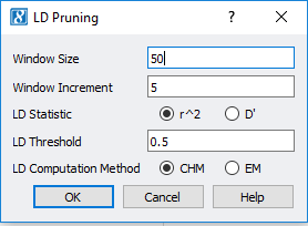
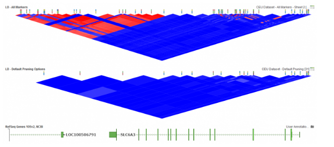
In SVS, LD pruning can be accessed by going to Genotype>Quality Assurance and Utilities>LD Pruning. In the LD Pruning dialog, Figure 1, the default options are commonly used for basic pruning and can be customized. The first option is window size where a small window size can be used for smaller datasets and will make it, so LD between distant markers are compared. The window increment reflects how far the window is moved after each time LD is evaluated between pairs of markers. While the LD Threshold is set to define a point when a marker will become inactivated. In SVS, LD can also be plotted in GenomeBrowse to display the effects of pruning, see Figure 2 below. For more details on setting up LD pruning, click here.
Why does Relatedness matter?
Relatedness is important to take into consideration as the premise of GWAS is that the observed genotypes are from unrelated samples in a random mating population. Deviations from this might include family-relatedness and inbreeding. Other factors include duplicate samples from platting errors, duplicate samples from one of a pair of genotyping chips, or sample contamination. To asses for these factors, we can use a feature known as Identity by Descent (IBD).
What is Identity by Descent (IBD)?
IBD is a measure of how many alleles at any marker in each of the two samples came from the same ancestral chromosome. To estimate the degree of IBD, SVS implements three probability coefficients: Z=0, Z=1, and Z=2. These probabilities reflect the level of sharing 0, 1, or 2 alleles that are identical by descent, respectively. We also use PI, which is the probable number of shared alleles at any given marker as well as Identity by State (IBS). IBS is a measure of how many alleles at any marker in each of the two samples happen to be the same. Together IBD will find samples related to one another or detect sample contamination, which can be used to further subset your data. More details here.
How do you access IBD?
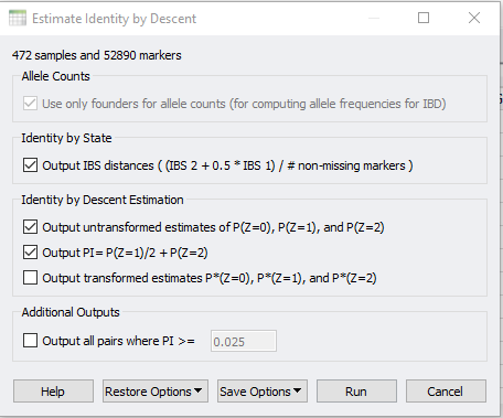
In SVS, IBD can be accessed from your pruned SNP dataset by going to Genotype>Quality Assurance and Utilities>Identity by Descent Estimation. After selecting the values in the dialog shown in Figure 3, the output will be two spreadsheets, one of which is IBD Estimate: Estimated PI. This spreadsheet, shown in Figure 4, is an N x N table where N is the number of samples in the dataset. To gain a better idea of sample relatedness, this information can be plotted in a heatmap (Figure 5).
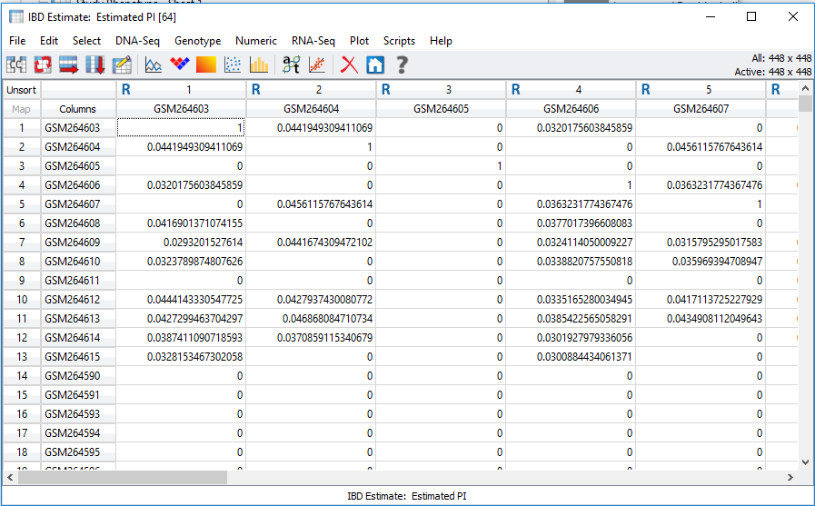
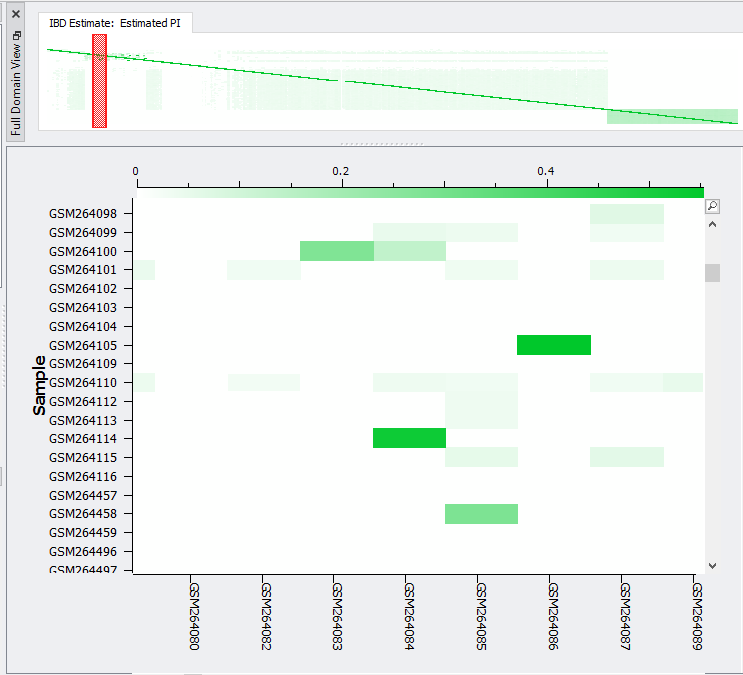
Fig 5. Heat-map of IBD showing the relatedness level colored comparison between samples.
The heatmap of IBD will present a colored profile sample pair relatedness, which if high can be subsequently removed from your study. To remove samples, you can use the Additional Outputs option to output all sample pairs with a minimum PI value. This will give a list of samples with high PI that can be removed from your cohort.
LD pruning and filtering for sample relatedness are important for reducing redundant data and for preventing bias that could skew your association tests. With these quality assurance steps, you are now ready to perform Principle Component Analysis (PCA). Stay tuned as PCA will be the focus of our next blog.
- William Bus, Jason Moore. Chapter 11: Genome Wide Association Studies. PLOS Computational Biology. December 2012: Volume 8, issue 12.