Curious about how coverage statistics can be used in conjunction with VarSeq? Evaluating the coverage over target regions or whole genomes is essential whether you are working with variant or CNV analysis. VarSeq has had the capability to compute sample level coverage statistics for some time now, but in the 2.2.2 release of VarSeq, there are some new features that I want to point out and discuss. It is no secret that coverage analysis is an important step in evaluating the quality of your data. In principle, there are two goals when analyzing the coverage of your samples:
- Make sure that there is sufficient coverage so that you can be confident in variant and CNV calls.
- Check that variants or CNVs were not undetected in regions due to an insufficient number of reads.
VarSeq offers users the ability to compute sample level coverage statistics based on the quality-filtered pileup depth from the sample BAM file. Total coverage and strand-based coverage is computed across user-defined regions in the case of whole exomes or gene panels or fixed-width bins in the case of whole-genome analysis.
In this blog, I will illustrate an example of coverage analysis for variants and CNVs for a whole-exome dataset pointing to ways to implement the new features that have been added to the algorithms. VarSeq has two algorithms available that can be used to compute coverage from the sample BAM file; the Targeted Region Coverage Algorithm and the Binned Region Coverage Algorithm. These algorithms can be added to your project by going to Add-> Computed Data (Figure 1).

If you are working with whole exomes or gene panel data, the Targeted Region Coverage algorithm is ideal as you can define the regions in which you would like to compute coverage statistics using a BED file. If you are working with whole genome samples, the Binned Region Coverage algorithm allows you to define the bin size to compute coverage across the whole genome. In either case, if you are using VarSeq to call CNVs, these regions or bins that are defined within the coverage algorithms will be the same regions that are used to call CNVs.
With some of the basics covered I think we are ready to jump into an example. At this point, I have imported my sample VCF and BAM files for whole-exome samples. However, I do not have a BED file to use for the Targeted Region Coverage algorithm. One of the additional features that have been added to VarSeq is that you can use RefSeq Genes to generate a BED file. What is a BED file exactly? The BED file merely contains the chromosome number and start and stop positions for either all exons or perhaps a target panel of genes. In my case, I want to create a BED file for a hereditary cancer-targeted gene panel with a 5bp padding surrounding each exon. To do this, I will start by going to Tools->Manage Data Sources, then choose RefSeq Genes from the list and click Export (Figure 2).
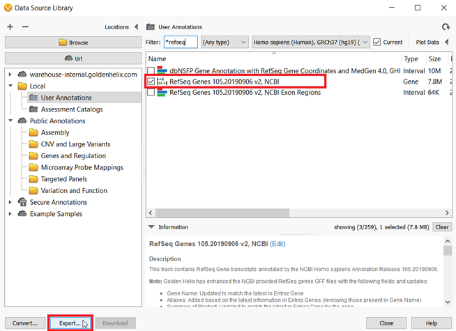
Figure 2: From the Data Source Window, RefSeq Genes can be exported to create BED files
Then choose Export Exons from the list and click Export (Figure 3).

Figure 3: There are a few different options to export annotation sources from VarSeq, as a text file, Excel file, etc. To create a BED file, choose the Export Exons option.
I mentioned that I want to include a few additional base pairs surrounding the exons, so in the next dialog window, I can set the +/- 5bp padding. Then I will add the genes in my hereditary cancer gene panel into the “Filter to Only Genes” window (Figure 4).
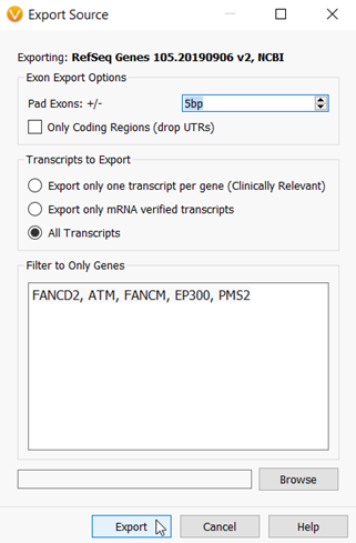
Figure 4: The Export dialog in which you can choose to export all genes and exons, or subset the export to a targeted gene panel with optional padding around the exons.
The final step is to convert the file within VarSeq so it can be used to calculate coverage. From the Manage Data Sources window, click on the Convert icon in the bottom left-hand corner. Next, add in the file that was just created. Then follow the prompts until the file conversion is complete (Figure 5).

Now I am ready to run the Targeted Region Coverage algorithm in our project (Figure 1). The first input that the algorithm needs is the BED file defining those regions in which I wish to compute the coverage statistics. As you can see in figure 5, I have selected the Hereditary Cancer BED file that I created and set three custom thresholds.
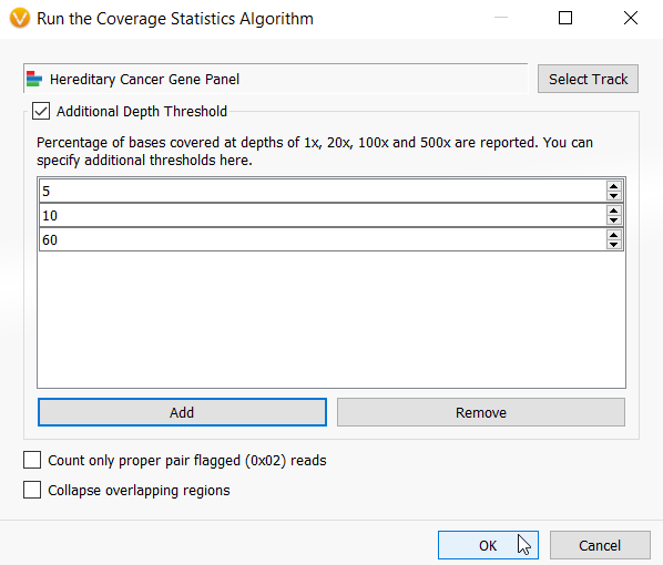
Figure 5: Interface for selecting the inputs for the Targeted Region Coverage algorithm including selecting the BED file and defining any custom threshold calculations.
A nice addition to the Coverage algorithms in VarSeq 2.2.2 is that you can define custom thresholds to calculate coverage. This was inspired by many VarSeq user requests and comes in handy particularly for generating clinical reports. It is not uncommon that a report must contain a list of failed targets at a certain coverage depth. The Coverage Statistics algorithms automatically calculate statistics at 1x, 20x, 100x and 500x depths, but now you can add an infinite number of custom thresholds to your analysis (Figure 5).
There are several calculations and metrics produced from the algorithm and those outputs can be analyzed within the coverage regions table. The coverage regions table, much the like variant table, can also be annotated with a number of different sources and algorithms and those fields can be used to filter the regions. As an example, I have filtered the target regions to the regions in my sample with a minimum depth of zero. (Figure 6).
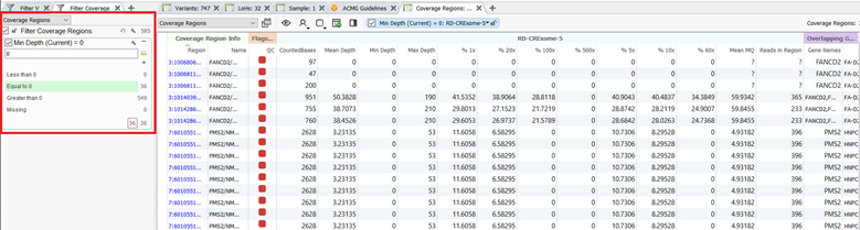
After filtering down to the regions with zero coverage, I can see that I have 36 regions within my hereditary cancer gene panel that have low-quality exon coverage. I can now utilize another new feature that has been added to the coverage regions algorithms and flag these regions as low quality to include in my clinical report. These flagged regions are shown by the red boxes in figure 6.
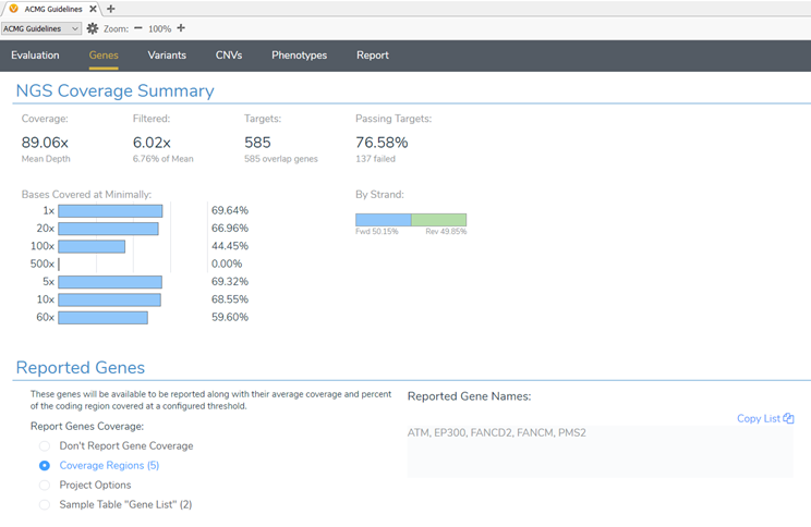
The coverage regions table is a great place to start analyzing the coverage of a sample. However, you can get visual summaries and evaluate coverage not only at a gene level but also per exon through VSClinical. VSClinical AMP has had this feature incorporated into the workflow for some time now. In the 2.2.2 VarSeq release, these coverage summaries and statistics are now available for the ACMG Guideline workflow as well! (Figure 7).
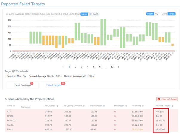
The final step in wrapping up the evaluation of the coverage statistics for the sample is to analyze the failed target regions that I flagged from the project to include these regions in the clinical report. Figure 8 shows the coverage for each exon or target from the hereditary cancer gene panel. The 36 failed targets are those flagged from the project and you can see how many of those targets were in each gene. Alternatively, you can use the Target QC Thresholds to define minimum required coverage, desired coverage, and desired average mapping Quality (MQ) to report failed target regions.
I hope this blog helps with understanding how you can use VarSeq and VSClinical to analyze the coverage statistics of your data. The new features that have been added to the coverage statistics algorithms emphasize the importance of the essential step to ensure quality data is being used as quality results are being reported. If you have any questions about coverage analysis within VarSeq, the field application scientist team at Golden Helix will be happy to help! Feel free to check out some of our other blogs that always contain important news and updates for the next-gen sequencing community.