Global population frequency catalogs like 1kG Phase 3, gnomAD, DGV, and others are excellent resources for identifying rare variants in your copy number variant (CNV) analysis. However, they are not exhaustive, and the reality is a lot of variants that are missing from global population frequency catalogs are still common variants. At the same time, CNVs that are identified by even robust callers can turn out to be artifacts. Therefore, it is extremely useful to be able to add another layer of variant tracking and filtering by creating your own CNV frequency catalog, and we have just the tool for you! VarSeq gives users the means to create their own CNV frequency catalog using our assessment catalog feature. The focus of this blog is to teach our users how to add this powerful component to their filtering strategy.

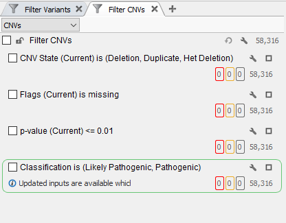
In this example of a CNV analysis using whole-exome sequencing data, it is already apparent that there more CNVs called than could possibly be clinically relevant (Figure 1). This is where global population frequency databases come in as a tertiary analysis tool to scrub out common variants. In addition, you can use our assessment catalogs to create your own CNV frequency database to track variants that are specific to your population being analyzed, identify common variants in your population, and also identify those regions specific to your analysis that are producing CNV calling artifacts.

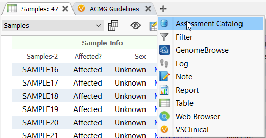
In order to get started with a CNV frequency catalog, it is always a good idea to do a cohort analysis. In this example, we will create a CNV frequency catalog using a cohort of 47 samples (Figure 2).

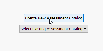
To begin, open up an assessment catalog from the tables drop-down menu. From the two options that appear choose “Create New Assessment Catalog”.

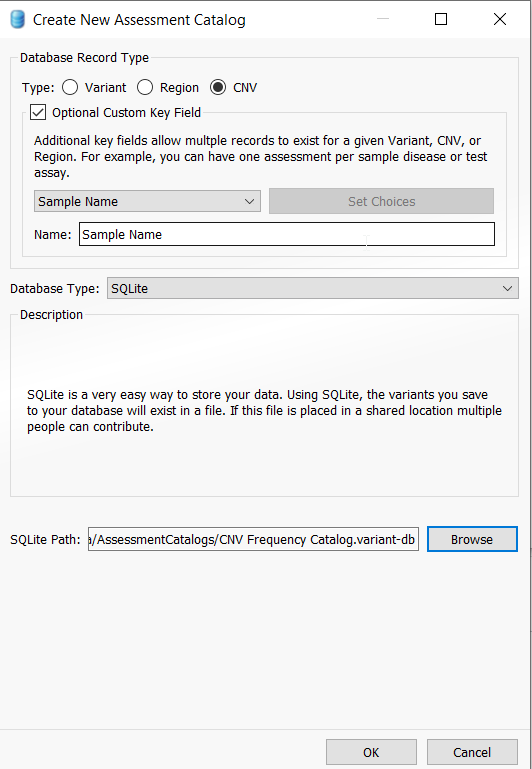
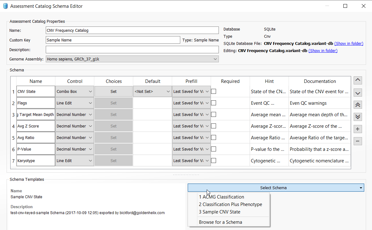
This action will pull up the catalog creation menu and you will appreciate that there are several types of assessment catalogs that a user can create, including the CNV frequency catalog. Select CNV, and also ensure that the Optional Custom Key Field is checked. Leave Sample Name and SQLite as the defaults (note that a user with access to VarSeq Warehouse can choose to create a Warehouse catalog instead of using SQLite). Lastly, choose a location for your catalog by selecting “Browse“, give your CNV frequency catalog a specific name and then click “OK” to save the catalog.

Once the catalog is saved, you will select the schema and further define the fields you would like to capture for your CNV frequency catalog. VarSeq comes with a predefined schema as a guide, but users can add any custom field they wish to capture. For this example, we are going to stick with the default fields for the Sample CNV State schema selected from the drop-down menu. Other options for catalogs include those based on the variant classification and phenotype. For example, you could create a catalog just for “Pathogenic CNVs”, as explained in one of our previous blogs.

Next, you’ll notice the catalog now presented as a tab in the VarSeq view. The next step in setting up the capture of all our CNVs is to utilize the single filter “CNV State” which is seen in the CNV table below. Conceptually, we are going to pass through each sample in the project and capture all CNVs detected in each sample. This will become obvious when we get to the end of these instructions.

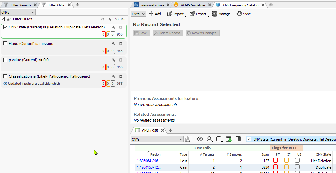
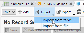
Once the filter for CNV State is defined, click the Import option in the assessment catalog and select Import from table.

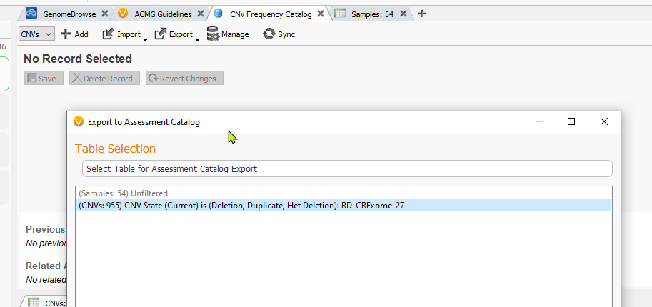
Choose to import the CNVs’ current filtered status for the single CNV State filter shown above (i.e. capture the total number of CNVs for this given sample which is 955).

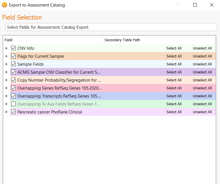
The next menu will present you with all of the fields available in the CNV table, but not all of these fields will be mapped to the catalog once we start the import process. All that is needed at this step is to click Next.

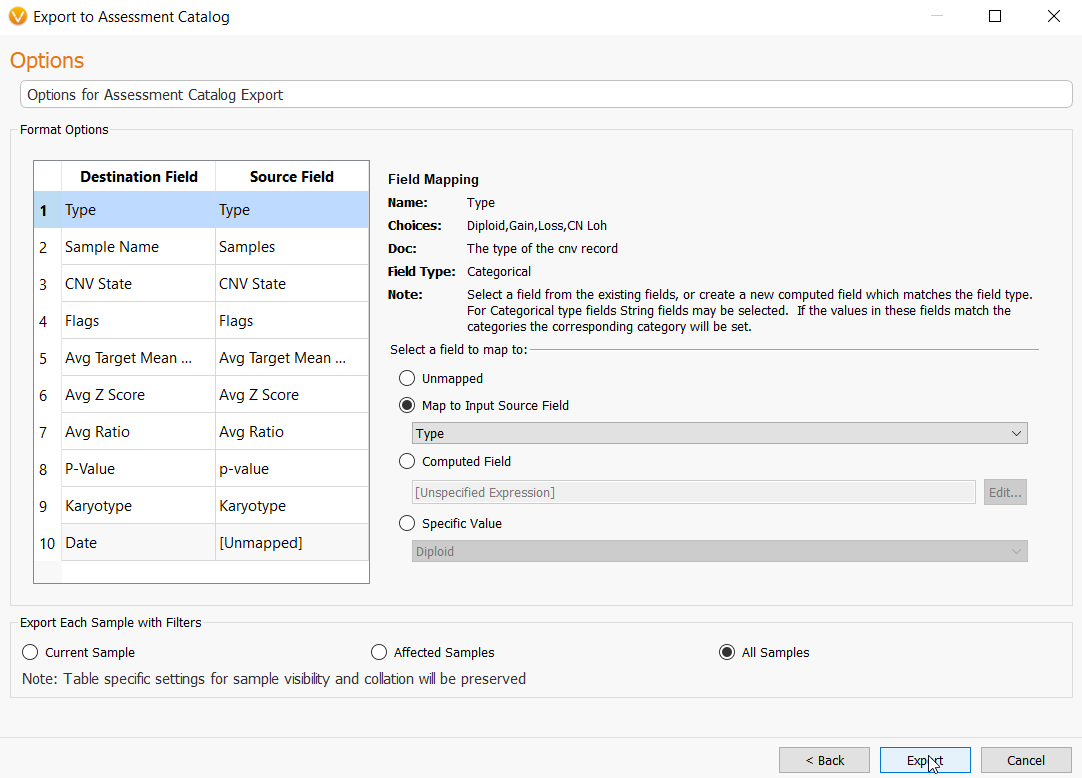
In this next step, the user may need to match source field and destination fields. In most cases, these fields may be automatically mapped correctly to their matched field. However, some manual selection may be necessary. You can do this very easily by going to Map to Input Source Field under the Select a field to map to section and choosing the correct field from the drop-down menu. Lastly, choose the option to import CNVs from every sample in the project by selecting All Samples, then Export, and this will create your CNV frequency catalog.

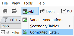
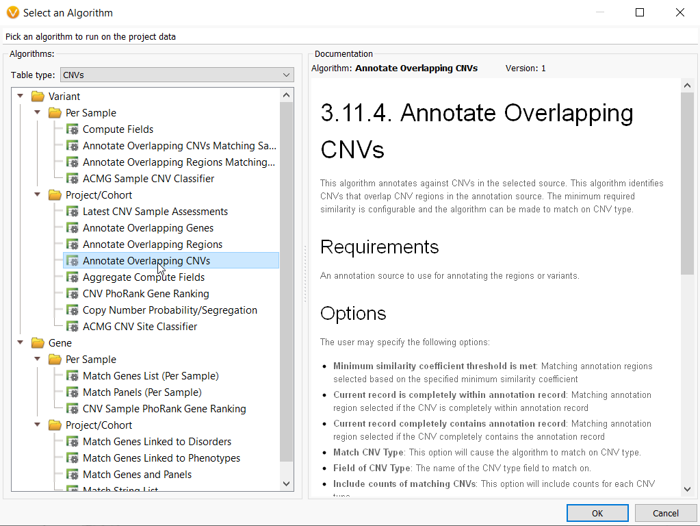
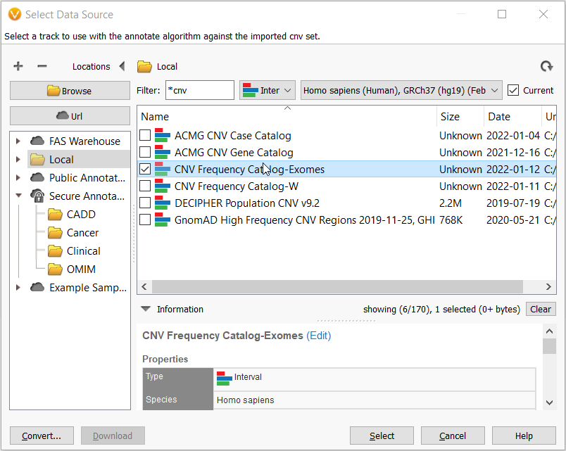
Now that the CNV frequency catalog has been created and CNVs have been added to it, you can use this new catalog as an annotation source. On the top left toolbar click the Add icon and select computed data (Figure 10a) then choose the Annotate overlapping CNVs algorithm.

Then in the Select Data Source window, navigate to your Local folder and here you get to choose the CNV frequency catalog that you just made!

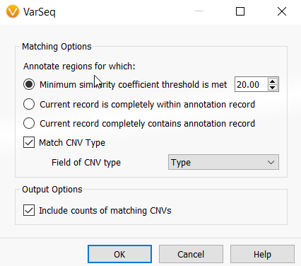
This will bring up a Matching Options window (Figure 12). The Minimum similarity coefficient is the minimum percentage overlap between a new CNV and any existing CNVs in your catalog that allows a CNV being analyzed to find a match in your CNV frequency catalog. You can adjust this coefficient to your preference, but 20% is a great starting point.

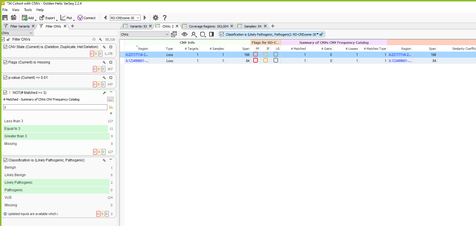
Once the CNV frequency catalog is added as an annotation in the CNV table, you can use specific fields in your filter chain to eliminate common CNVs that overlap the events seen in future samples. You can see in the image below (Figure 13), for this example, our sample initially had 1178 CNVs. We filtered down to 127 CNVs that are high quality using the Flags filter, and high confidence by filtering on p-value. Then we used our CNV frequency catalog to filter out those that are common among our exome cohort by using the # Matched field in the Summary of CNVs CNV Frequency Catalog section. In our filter chain, we invert this filter to remove 20 CNVs seen across 3 or more samples. Lastly, we honed in on 2 likely pathogenic candidate CNVs for this specific sample.

Another very informative way to use the CNV frequency catalog is to plot it in Genome Browse along with the CNV for your current sample. This allows you to visualize the overlap of CNVs in your catalog with the current CNV being analyzed, in terms of how many overlap and the scope or size of the overlap (Figure 14). Lastly, in your CNV frequency catalog tab, you can see the information about previous assessments being stored in your catalog. This includes CNV metrics, the name of the sample, date of capture, CNV state, and the user on your team that captured the assessment. You can see in this example of a common event, that seven CNVs overlapping this heterozygous deletion in GHR have already been captured in our assessment catalog.

Our assessment catalog tool is a powerful tool for cohort analysis. This feature enables users to track the frequencies of CNVs as they accumulate over multiple samples in your cohort. If you found this blog useful for your analysis, you can head over to our How to’s and advanced workflows section for more blogs like this with detailed instructions on a number of features that VarSeq offers. As always, if you need help with building your own CNV frequency catalog or any other questions about our software products, please reach out to us at support@goldenhelix.com.