
Learn how VarSeq revolutionizes NGS workflows by enabling the integration of comprehensive internal databases, allowing bioinformaticians to create custom pipelines and maximize data analysis efficiency.
Are you a current (or future) VarSeq user with a perfect, comprehensive, internal database you simply can’t part with and can’t replicate? Do you dream of coalescing many disparate workflows into a consistent, reliable pipeline? VarSeq has the tools to make these dreams a reality, and it plays well with others.
Many pipelines in one with VarSeq
Bioinformatic freedom is at the core of the VarSeq software suite. Our mission at Golden Helix is to enable our customers to leverage their own expertise in a consistent and fast way. This goal manifests in the flexibility at all levels of workflow design with VarSeq. We give our customers the tools and support they need to implement their own ideal NGS workflow, and we have seen all manner of customized, efficiently implemented pipelines designed using the VarSeq software suite. In this blog, we’ll focus on leveraging the tools available within VarSeq and externally to bring custom databases into VarSeq for filtration and annotation.
As anyone who’s enjoyed one of our webcasts or demos can attest, annotations are at the heart of a validated and comprehensive NGS workflow. While we provide a wealth of curated public and secure annotations to our users, bioinformatic freedom is central here as well, and users have several tools at their fingertips to customize existing databases and convert their own databases into files accessible to VarSeq. Of course, with great power comes great responsibility, and there is no one-size-fits-all solution to database conversion, given the diversity of custom databases in the wild. In this blog, we’ll address some of the expectations VarSeq has when converting external databases and how to get databases to that state using external tools. Astute users will also note that during this entire process, all of your hard-earned and meticulously curated data is kept on-premise, and nothing is shared externally.
Getting ready for the big dance: Formatting data for import into VarSeq
All custom databases are in different forms. Today, we’ll tackle a classification database stored as an Excel file. The exact steps may be different for other internal databases, but this process will outline the methodology and desired output well enough to replicate in most cases. Let’s start by examining the fields and their format in our Excel spreadsheet (Figure 1).
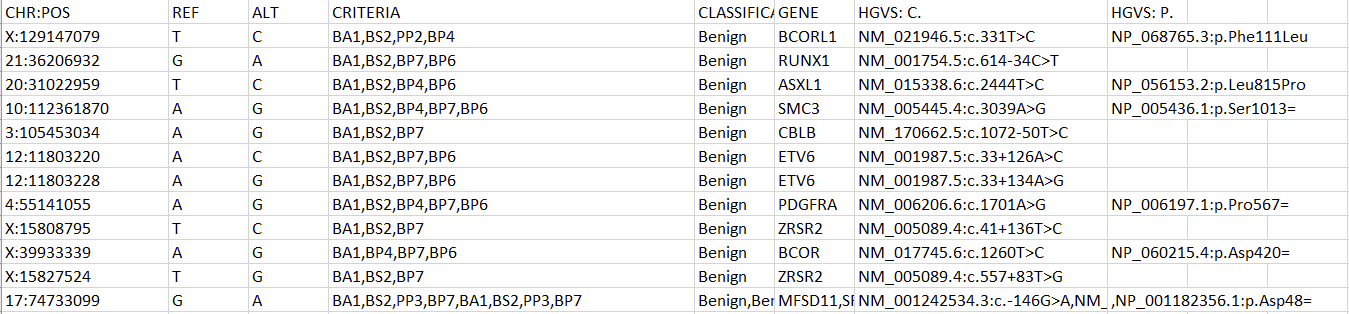
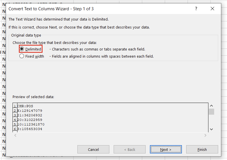
To create a variant annotation, VarSeq will expect a “Chromosome” field, a “Position” field, and a “Ref/Alt” field. We can use Excel tools to rework our columns to fit these expectations. Alternatively, VarSeq supports regular expressions during catalog conversion, but most users are more comfortable with Excel. Particularly savvy users might also prefer open-source tools like BCFtools or their own custom scripts to perform this conversion. For this example, let’s proceed with Excel. To start, we can split the “CHR:POS” column into two columns using the “Text to Columns” tool under the “Data” tab (Figure 2). Before doing this, we’ll also want to insert an empty column to the right of our “CHR:POS” to store the resultant extra column.

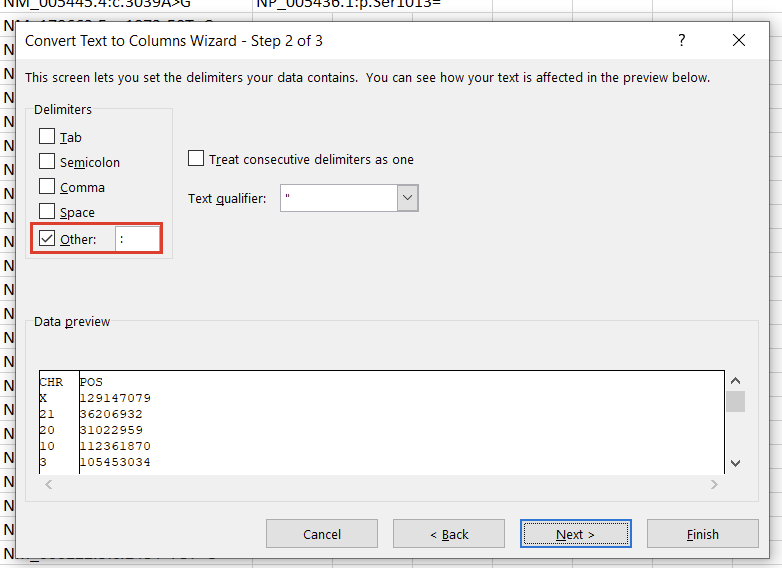
In the first window, we’ll want to select “Delimited” (Figure 3). Hit “Next,” then under “Delimiters,” choose “Other” and specify “:” (Figure 4). Clicking “Finish” will result in two columns, “CHR” and “POS.”
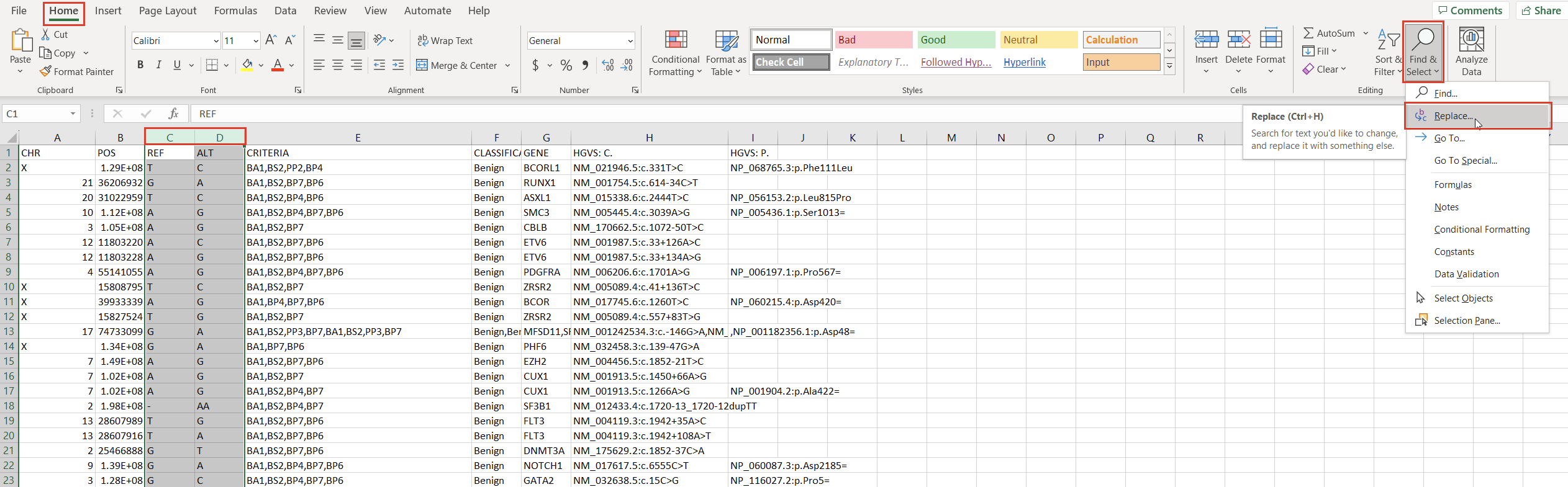
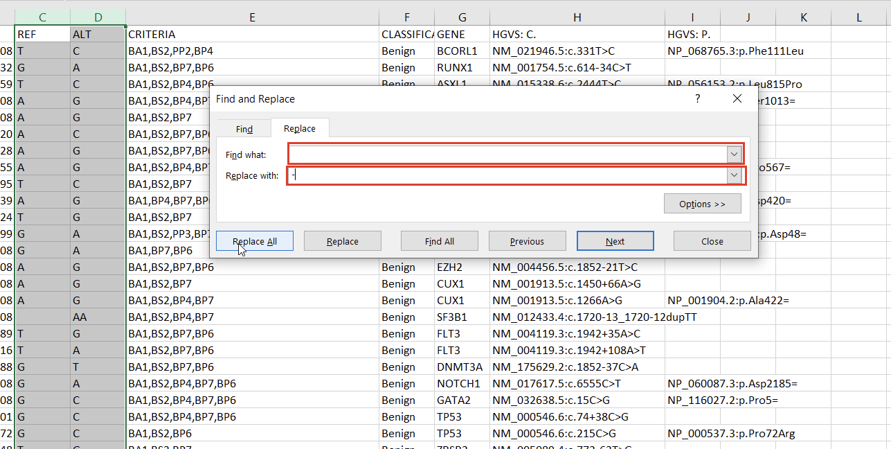
With the chromosome and position fields successfully split, we can address the reference and alternate fields. First, we notice that the deletions and insertions are represented with blank cells in this database. We can address this with a simple “Find & Replace” on the selected columns (Figures 5 & 6).
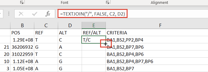
The next step to prepare our Excel spreadsheet for import into VarSeq as an annotation is creating a Ref/Alt field. We can do this by creating a new column to the right of the “ALT” column and placing the following formula in the second cell:
=TEXTJOIN("/", FALSE, C2, D2)
Double-clicking the “+” that appears in the bottom right of that cell will then apply the formula to the entire column (Figure 7).
Lastly, we need to provide a start and stop field. Position represents the 0-based start position. Let’s insert an additional column before the reference column and repeat the steps to produce the Ref/Alt column using the following formula:=(B2 + LEN(E2) - 1)
This will result in a stop position. The reason we subtract one is because the stop position is 1-based. We’ll touch on this a little later as well. Now, with our chromosome and position fields separated and our new Ref/Alt and stop fields, we’re now ready to transform our Excel spreadsheet into a VarSeq-readable annotation.
Same data, new look
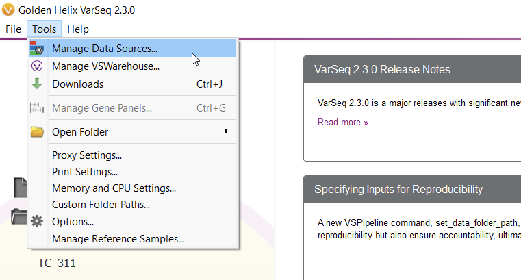
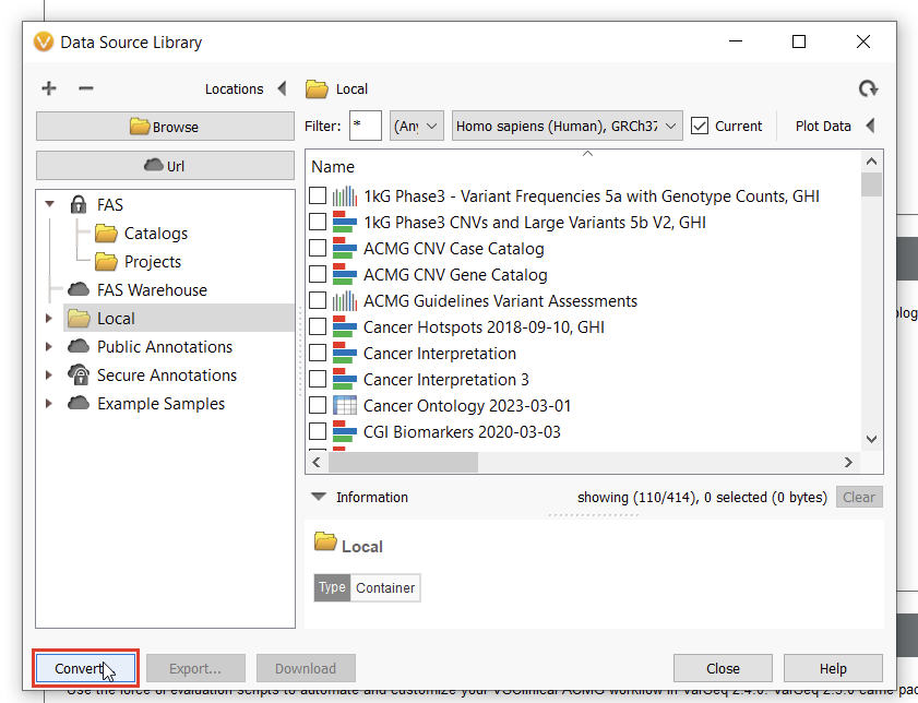
To start curating a new track, you’ll have to navigate to the Data Source Library in VarSeq, found under Tools > Manage Data Sources… (Figure 8). The window displayed represents all of the locally installed annotation tracks and catalogs available to you, as well as those hosted on our public and secure folders. Our journey today, however, regards a third option for database conversion, namely the “Convert” tool, found in the lower-left corner of the Data Source Library window (Figure 9).
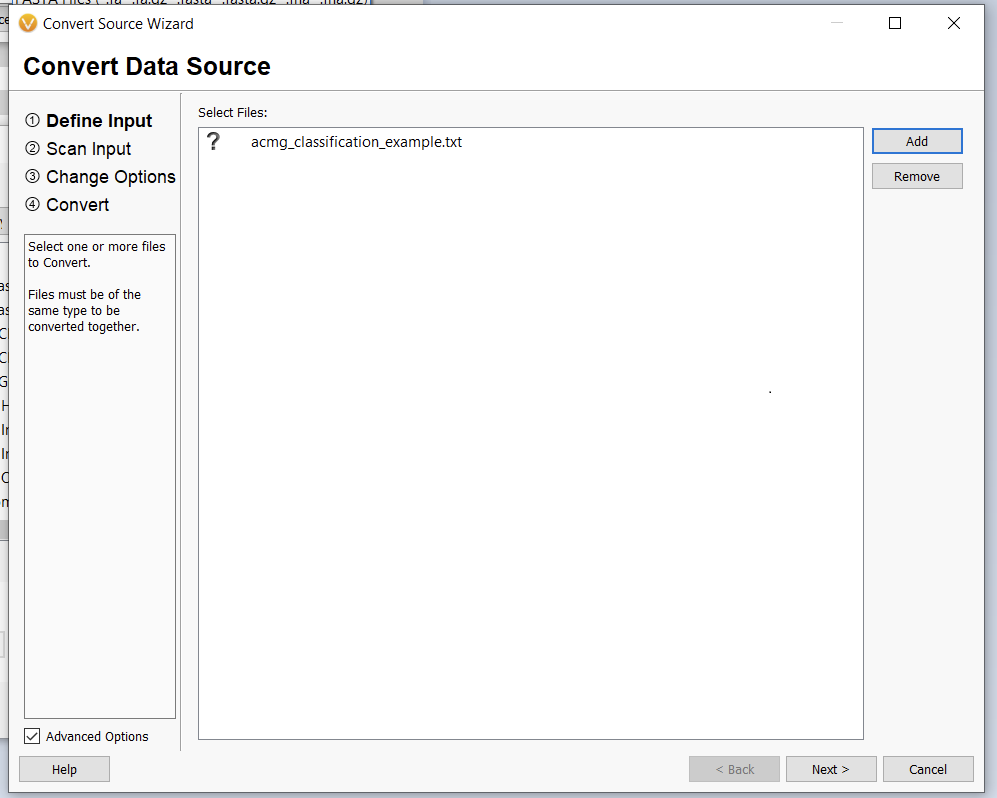
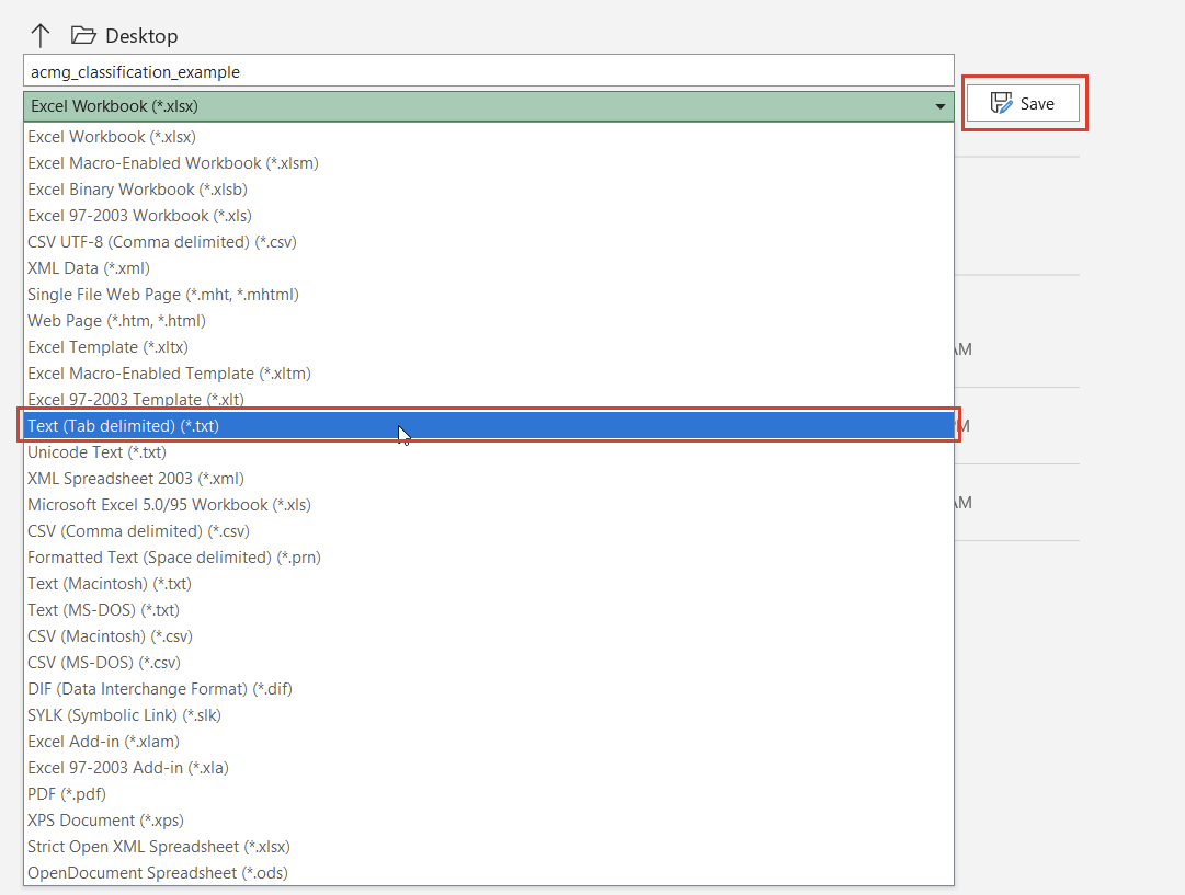
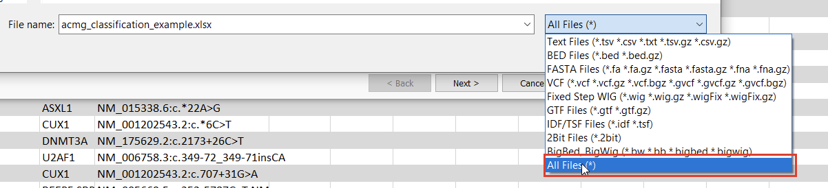
Once we click the “Convert” button, we can choose which source we’d like to bring in (Figure 10). Before importing, we’ll have to save our Excel spreadsheet as a text file (Figure 11), and we may also need to change the search criteria in File Explorer depending on the file extension you use (Figure 12).
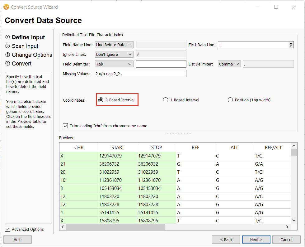
The next window allows us to change some of the input behavior. For instance, we can define whether or not there is a header consisting of a single line or if the interpreter should ignore lines starting with a specific character, such as a “#” in a VCF. The interpreter should also automatically detect the chromosome, start, and stop fields. We’ll worry about the Ref/Alt field in the next dialogue window. For now, we can select “0-based” (since we subtracted 1 from our stop field) and continue (Figure 13).
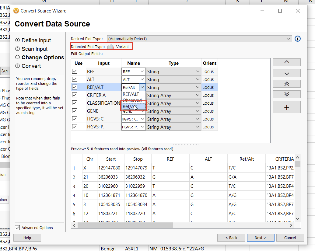
The next screen will allow us to define the fields we want to include in our annotation track. Here, we’ll need to specify the “Ref/Alt” field, after which the automatically-detected plot type should be “Variant” (Figure 14). Clicking “Next” will allow us to define the genome assembly. VarSeq will notify you if something doesn’t look right, but be sure to double-check that you’re selecting the correct assembly nonetheless. Finally, by clicking “Next” again, we can choose a name for our annotation track and then click “Convert” to bring our new track to life.
Once we’ve completed these steps, our new annotation track will be available in the Data Source Library and can be selected from any VarSeq project as an annotation source and used in filtering. Furthermore, the new annotation can be visualized in GenomeBrowse.
This guide is unfortunately not comprehensive but should be a good starting point for those looking to bring internal data into VarSeq as an annotation source. As always, our FAS team is more than happy to guide users through the intricacies of database conversion for even the most esoteric of legacy databases. We look forward to bringing your data under one umbrella and helping you make the most out of VarSeq!