Our software solutions and partners have brought dramatic improvements to the secondary and tertiary analysis stages of variant evaluation. Regarding secondary analysis, we’ve discussed increased efficiencies in speed and overall accuracy in the variant calling process with Sentieon. On the tertiary side, we have explored numerous workflows in VarSeq highlighting filtration to clinically relevant variants, as well as the automated ACMG and AMP guidelines in VSClinical. The purpose of this blog series is to address the post-analysis environment these processed variants are stored in. VarSeq provides a means for users to store their classified variant interpretations and easily leverage the captured data across future samples. Part I of this blog series covered the capture of variant classification run through the ACMG guidelines in VSClinical, but this strategy is also deployed in regard to copy number variants. In part II of this blog, we’ll be exploring how to capture classifications of CNVs detected in VarSeq, but also how to leverage a CNV frequency assessment catalog to remove CNV signals of high abundance to eliminate artifacts from the secondary analysis pipeline (i.e. false positive events).
In part I of this blog series, we focused on an assessment catalog built to store variant classifications and interpretations for SNV and indels processed through VSClinical. This is also true for the copy number variant capture as well. Users can build assessment catalogs to capture any kind of information they’d like from their variants. Whether it be tracking low coverage regions to optimize library prep or secondary analysis, remove artifact variants (false positives), or if wanting to build their own frequency catalogs. Figure 1 shows the options users have to build variant, region, or CNV level catalogs.
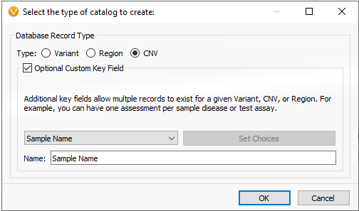
Figure 1. Building an assessment catalog for CNV/Regions/Variants while retaining unique sample identification.
Fortunately, VarSeq comes with a premade schema to help guide users in defining the fields they wish to capture. The example in Figure 2 shows the selection of the multiple schemas available which in this example we will be selecting the Sample CNV State. Selecting the CNV schema provided us with the majority of the fields necessary for sample CNV capture and there was an added field for classification in a multi-selection format for pathogenic, likely pathogenic, uncertain (default), likely benign, and benign.
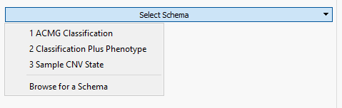
Figure 2. Optional schema prebuilt into VarSeq for creation of custom assessment catalogs.
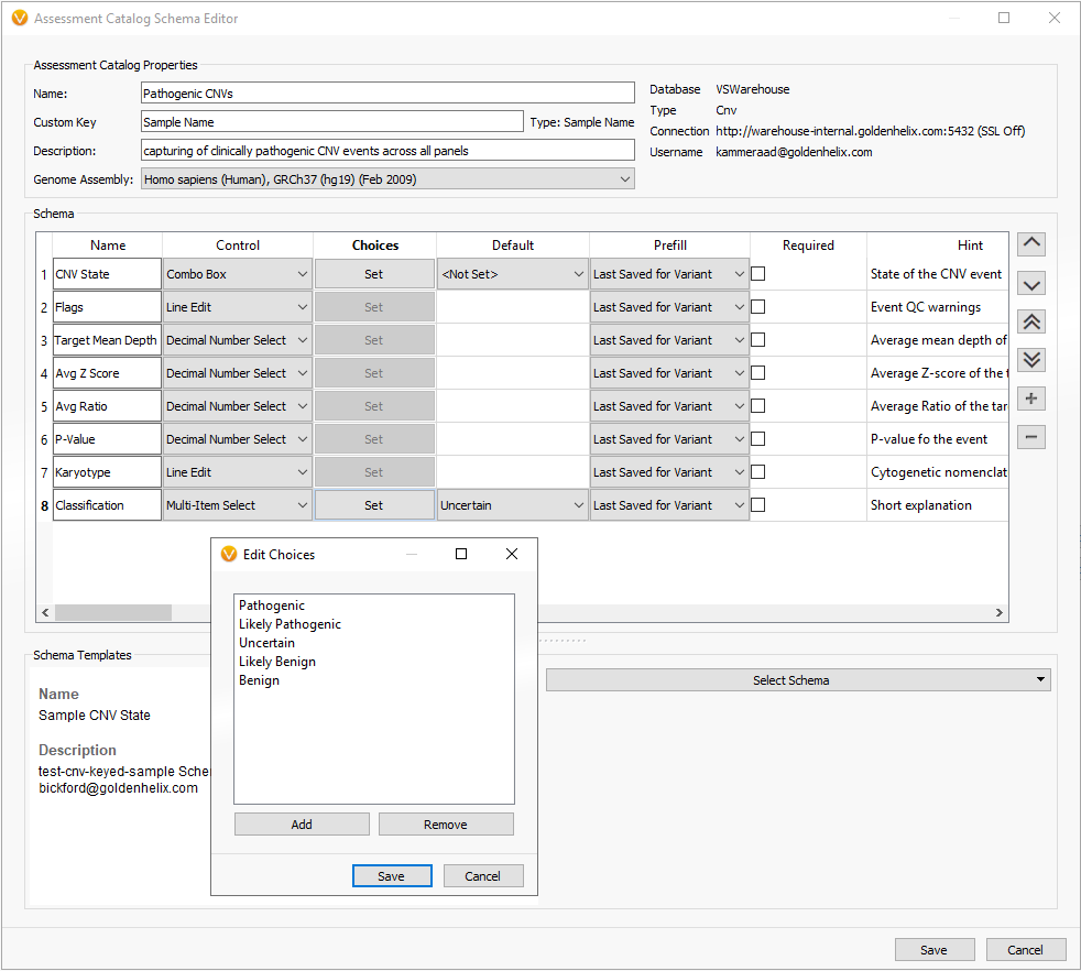
Figure 3. CNV based schema with additional field to capture classification of CNV event.
When filtering through the called CNVs, a single heterozygous deletion in this given sample was captured. The metrics supporting the CNV call are stored, classification decided, and interpretation built all using tools within the VarSeq interface (Figure 4a). Figure 4b shows the finalized stored content referencing not only the CNV call metrics and classification but also the user who captured the interpretation.
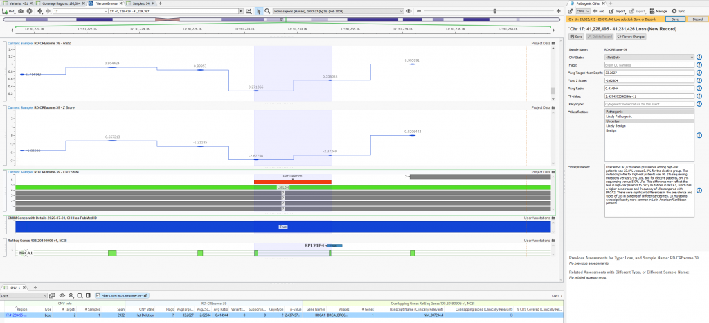
Figure 4a. Visualization of clinically relevant variants in VarSeq with the assessment catalog captured content on the right side.
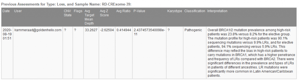
Figure 4b. Archived history of captured CNV showing CNV details, recorded classification, and author.

As mentioned earlier, users can create custom catalog for a variety of formats. What we have looked at thus far is a cataloging CNV classifications, but we also can build a CNV frequency catalog to help filter out noisy regions. One downside to using known germline CNV frequency catalogs (1KG Phase 3, gnomAD, ExAC, etc) is they only go so far in handling the CNV output from your library pre and secondary analysis pipeline. Each user will have unique considerations for their prep method and pipeline with the ultimate goal of wanting to easily filter out CNVs from these noisy regions. One easy way to represent this is with a plot (Figure 5) showing the overlap of any given CNV against a CNV frequency catalog. The question is, should I trust the het deletion call I see as output in the figure? It becomes pretty apparent that this is an artifact when I see that across all the samples I’ve run, there is a mix of high number of deletions and duplications over this region. In other words, this region may just be noisy and I can easily ignore CNVs overlapping regions like this from a filtering perspective.
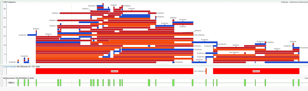
Figure 5. Heterozygous deletion called in Sample 39 aligned with an in-house CNV frequency catalog.
Again, each users’ workflow, data, samples, panel, overall pipeline is going to be unique. The conceptual nature of CNV detection is in itself a challenge but so is the design of the tertiary solution to handle the called events. This is especially true when dealing with whole exome level data. Golden Helix has proven its ability to not only accurately call the CNV events even down to a single exonic level, but also be a market leader in strategies for annotation and filtration down to clinically relevant variants. If you would like to setup your own CNV pipeline, please reach out to support@goldenhelix.com for a demo/training call.