SVS offers several options to conduct genome wide association tests and mixed linear models. At times, it can be challenging to decide which test, model, or adjustments to use when setting up your analysis. I want to briefly explore the options available in SVS for association tests, and mixed linear models to hopefully facilitate in understanding and choosing which options fit best with your data. Let’s begin by taking a look at the genotype association test menu options.
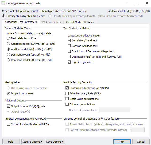
Figure 1 shows the genotype association tests window in SVS which offers a way of testing for genotypic association against either case/control status or a quantitative trait. There are several statistical measures that are available given the genotype model assumption that is chosen. For a few genetic models, you can choose to use stratification correction via Principal Component Analysis (PCA) or Genomic Control via the lambda inflation factor. With some tests, you may choose to drop missing values. However, there are also situations wherein you could use missing data values in your genotypes as predictors if you wanted to understand how much the response depends on these missing values. Before things get too complicated, I first want to explain the genetic models/tests and then we can deep dive into the type of test available for each model.
For any association test, you want to start by selecting the genetic model or test. Figure 1 shows how we can choose either the basic allelic tests, genotype tests, additive, dominant, or recessive models.
In the explanations of these models or tests, D represents the minor allele and d represents the major allele.
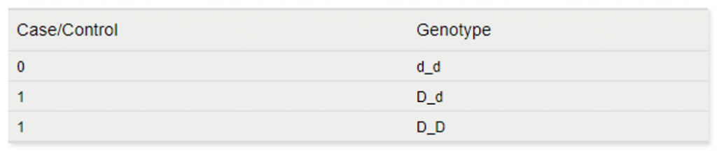
- Basic Allelic Tests– For a basic allelic test, the genotypes dd, Dd, and DD are fixed into pairs of alleles d and d, D and d, or D and D. Both alleles of each subject’s genotype are considered to correspond to the same value of the dependent variable, like a quantitative or case control phenotype. The associations with these individual alleles are then tested. They say a picture is worth a thousand words, so here is a quick example. Consider the following genotypes for three individuals for the same marker:
The basic allele test would translate these genotypes to the following to run the association test:
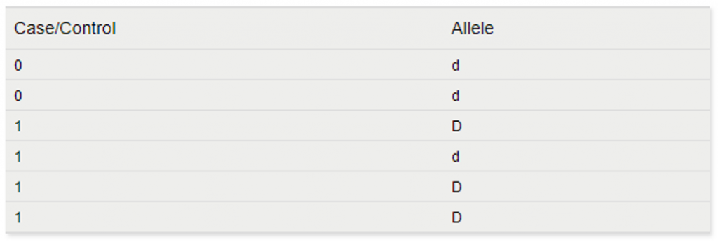
The advantage of this test model is that the number of observations has doubled. However, the genotype-specific information (which alleles are paired together) is ignored. Also, PCA is not available for this model.
- Genotypic Tests– Genotypic tests test on the genotypes dd, Dd, and DD without any regard to “order”, allelic count or allelic paring. What this means is that the risk factor for case vs control status associated with the genotype for a specific marker would not be considered. For example if the heterozygous allele state indicates an increased risk for disease by x number of folds for each Dd genotype and by a 2x fold for genotype dd then the genotypic test model would not take into account the penetrance of the disease. However, the additive model does.
The next three models can be used whether the alleles are being classified according to allele frequency or the reference/alternate alleles.
- Additive Model– In this model the association depends additively on the minor allele. So that means having two minor alleles (DD) vs having no minor alleles (dd) is twice as likely to affect the outcome in a certain direction than having just one minor allele (Dd) vs no minor alleles (dd).
- Dominant Model– If the alleles are classified according to allele frequency, this model tests the association of having at least one minor allele D (either Dd or DD) versus not having it al (dd). This model works similarly if the alleles are classified according the reference/alternate alleles.
- Recessive Model– This model specifically tests the association of having the minor allele D as both alleles (DD) versus having at least on major allele d (dd or Dd).
Once you have selected the model you would like to use, you can choose which test statistic is appropriate for your data. The table below summarizes the test statistic and the scenarios to run each test.
| Test Statistic | Missing Values must be dropped | Variables | Genetic Model | PCA Available | Description |
|---|---|---|---|---|---|
| Correlation/Trend Test | Yes | Case/Control and Quantitative | All genetic models except genotypic test | Yes | Shows the p-value for the dependent variable having a correlation with the input data. |
| Armitage Trend Test | Yes | Case/Control | Additive model only | No | The case vs control having a trend which depends on the count of the alt allele. |
| Exact Form of Armitage Test | Yes | Case/Control | Additive model only | No | More computationally expensive than the normal Armitage Test, and it avoid the chi-square approximation. |
| Chi-Squared Test | No | Case/Control | All genetic models except the additive model | No | Two contingency tables of observed vs expected with all possible variations of the select genetic model in one direction vs case/control status in the other direction |
| Chi-Squared Test with Yates’ Correction | No | Case/Control | All genetic models except the additive model | No | Just like Chi-Squared Test but the Yates correction subtracts 0.5 from the absolute magnitude of the difference between observed and expected values before squaring. Use when data is discrete integer rather than continuous. |
| Fisher’s Exact Test | No | Case/Control | All genetic models except the additive model | No | The probability of having a contingency table more extreme than the one observed assuming equal probability of any permutation of the dependent variable. Avoids the chi-square approximation. |
| Odds Ratios with Confidence Limits | Yes | Case/Control | All genetic models except the genotypic tests | No | The odds ratios indicate the intensity of the association. If two ratios are the same, then the additive model is valid. If the ratios are very different, then another model may better describe the data. |
| F-Test | No | Quantitative | All genetic models except the additive model | No | Tests whether the distributions of the dependent variable within each category are significantly different between the categories of the independent variable |
| Logistic/Linear Regression | Yes | Quantitative (real or integer values) | All genetic models except the genotypic tests | Yes- For Linear Regression | Linear reg- a line is fit to the response and an associated p value for the goodness of fit. Logistic reg- when the dependent variable is a binary trait and a curve is fit to the predictor and a p value is computed for goodness of fit. |
Briefly, before moving on to mixed linear model analysis, I want to mention the multiple testing corrections. When you are testing multiple hypotheses, these corrections are meant to ensure that a good test static value was not obtained by chance alone. The two that I want to discuss are the Bonferroni Adjustment and the False Discovery Rate (FDR). Both are particularly useful in logistic regression analysis and can also be used with mixed linear models.
The Bonferroni Adjustment is a conservative value that aims to eliminate the probability that this test would have obtained the same value by chance at least once from all the times the test was performed. It multiplies each individual p-value by the number of times the test was performed. Finally, the False Discovery Rate option can be used to calculate the FDR for each statistical test selected and can be interpreted as “ What would the rate of false positive be if I accepted all of the tests whose p-value is at or below the p-value of this test?”
Association tests are great for determining the relationship between a variable. However, mixed models are useful when the data has more than one source of variability and they take into consideration both fixed and random effects. What do I mean by fixed and random effects? Before I explain this in detail, I want to reference the SVS mixed linear model parameters to walk us through how to set up our analysis (Figure 2).
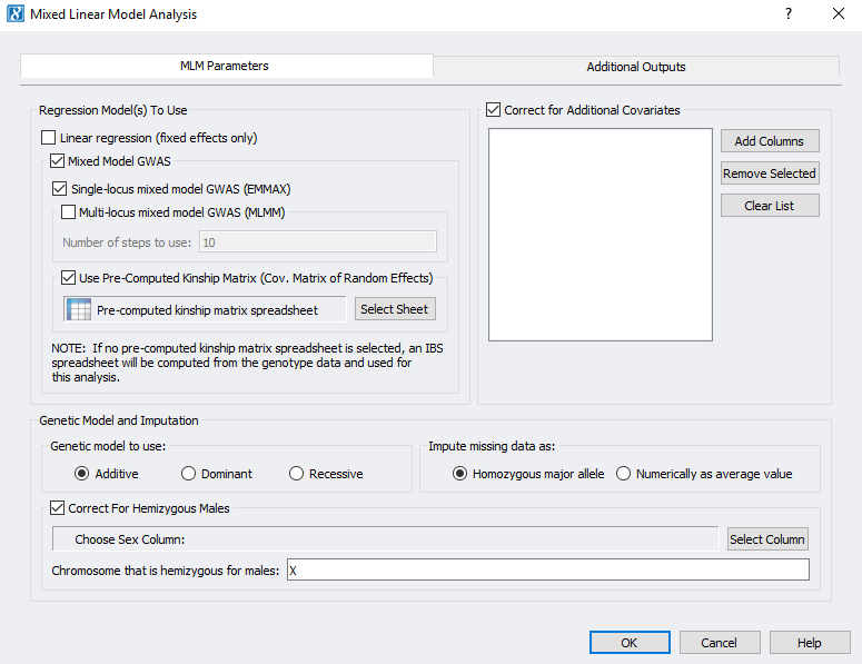
The first decision that you will need to make is which regression model to use. The linear regression is for fixed effects only. Just about any independent variable (categorical, integers, real values, binary, genotype markers, etc) can be a fixed effect in regression analysis and can be included in the model as fixed covariates. In a fixed effect model the idea is that whatever effects omitted variables have on the subject will have the same effect later.
A random effect models will account for any variables that may have been omitted or omitted variable that are uncorrelated with variables in the model. It will produce estimates for the coefficients, use all data available, and minimize standard error. There are two options for mixed linear models that incorporate random effects; GWAS mixed linear model with a single locus (EMMAX) and multi locus (MLMM).
Both GWAS mixed linear models use a kinship matrix to correct for cryptic relatedness (either a precomputed kinship matrix or an identity by state kinship matrix) as the random effect and the regression analysis is performed directly on genotypic data. These tests can also account for fixed effects in the model. When you include fixed effects in the model by correcting for covariates, these variables are not included in the analysis. A different way to think of this is to “correct out” the effects of an independent variable.
The next step is to decide if your dependent variable/trait is controlled by several markers that have a large effect on the data. If this scenario is true for your dataset, a multi-locus mixed linear model can be used. Essentially, a mixed linear model is a series of single locus regressions (EMMAX) in a stepwise fashion. First you will set up a model that includes fixed effects and covariates just like you would set up single locus regression. Then, the MLMM will scan all the markers that were not specified as covariates and select the most significant marker to be a new fixed effect (covariate). This step will repeat in what is called forward inclusion determined by the number of steps specified in the model. In figure 2 this number is 10. Next the MLMM will remove the specified markers from the fixed effects and scan only one marker at a time. The marker that is the least significant will be eliminated, creating a new model. These steps are referred to as backward elimination.
Additional parameters to set whether you are performing EMMAX or MLMM are to choose the genetic model, imputation, and correction for hemizygous males. The genetic models are the same Additive, Dominant, and Recessive models that were described for the association tests.
There are two options for imputing missing genotypes. The first is to use the homozygous major allele which will set missing genotypes to zero. Alternatively, if you are using numerically genotyped data you will impute the genotypes numerically as an averaged value, which will take the average of the non-missing genotypes values for each marker to recode the missing genotypes.
Finally, to correct for hemizygous males, there must be non-missing data for both males and females for a given marker. Then averages for males and females are applied separately.
One last thing I want to mention for setting up a mixed linear model in SVS is that you can still include the Bonferroni test correction and False discovery rate via the additional outputs. There are few other optional outputs in this menu that you can explore as well such as output to generate P-P plots or genotype statistics. If you have questions about any of these additional outputs, please reach out to us at support@goldenhelix.com and we will gladly assist.
Hopefully, this blog has made conducting and understanding association tests and mixed linear models within SVS a little bit easier. However, the Field Application Scientist Team at Golden Helix is always available to answers questions and help set up your analysis in the software. Additionally, there are tutorials for conducting both GWAS and mixed linear model analyses in SVS that can be very helpful. Links to those tutorials can be found here.