A Step-by-Step Guide to Creating a BED File from RefSeq for Accurate Data Analysis

Our FAS team has received a flurry of inquiries recently, asking how to run coverage statistics on their projects without a pre-defined BED file. We’re here to help! To analyze sample coverage statistics, you’ll need a BAM or CRAM file that displays the read depth coverage for your samples. But don’t worry, even if you don’t have a BED file, we have a solution for you. In this guide, we’ll take you through the process of creating a BED file from RefSeq with ease, converting it into an interval track, and setting you up for success with your sample coverage statistics analysis.

Step 1: Associate Alignment File

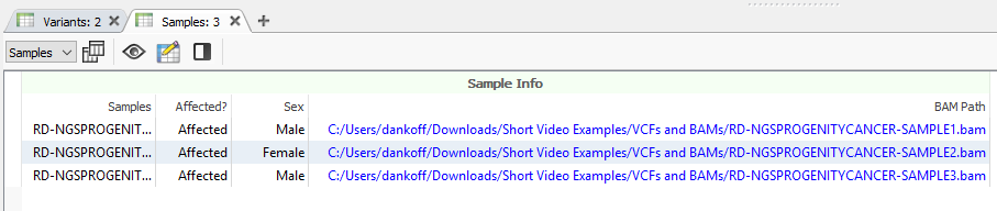
As mentioned above, you will need to have a BAM or CRAM file associated with the samples in your project, as seen below while looking at the Samples table (Figure 1).

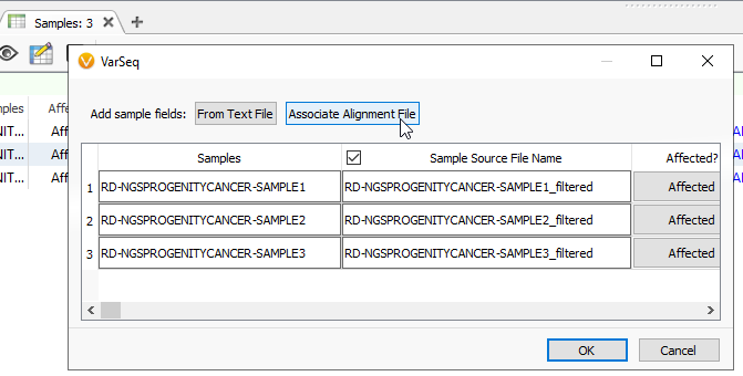
You can associate alignment files while first creating your project. Alternatively, if you have forgotten that step while building the project, you can edit the information into the Samples table. Click the blue spreadsheet button, and it will pull up this familiar dialog. Here, click the Associate Alignment File button (Figure 2). If your BAM or CRAM is located in the same file as your VCF and called by the same name, VarSeq will likely find the path on its own. Otherwise, you will be able to search manually for the alignment file.

Step 2: Download RefSeq Exons

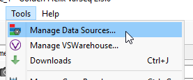
Now that the Alignment Files are associated, we can progress to making a BED file and ultimately running Coverage Statistics. First, go to Tools > Manage Data Sources (Figure 3).

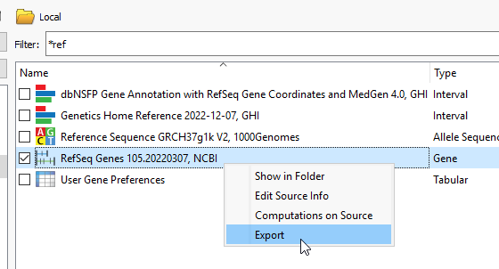
The next step is to bring in RefSeq and this will likely already be locally downloaded. A FAS note here- While we commonly use RefSeq to build these interval tracks, you can use other gene sources, like Ensembl. Right click on the source, and say Export (Figure 4).

Be sure to Export Exons (Figure 5).

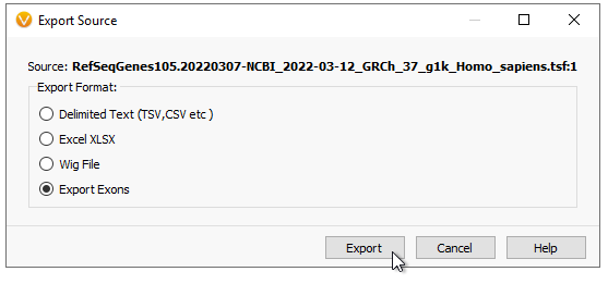
At this point, you have options (Figure 6). You can pick to export to exon coding regions, drop UTRs, or pad the export depth from the exon boundary. You can pick which transcripts you want to export, and if you want to export a subset of specific genes. Here I am exporting a very small panel searching for Breast and Ovarian Cancer variants. Make sure to use the RefSeq gene names to designate genes (or Ensembl names if using that track). Hit Browse to give it a name and pick a download location, then hit Export.

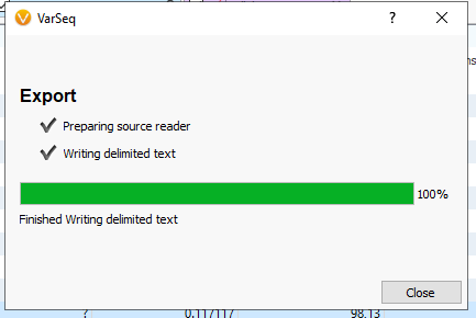
Depending on the size of the file, your export time will vary, but should run quickly (Figure 7). Hit close when the export reaches 100%.

Step 3: Converting from BED to TSF format (Interval Track Time!)

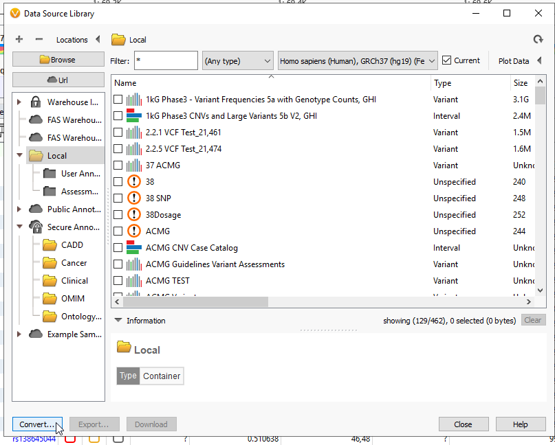
Your genes of interest have been exported as a BED file. The next step will be to convert that file to a TSF. Head back to Tools > Manage Data Sources… Then click on the Convert Wizard (Figure 8).

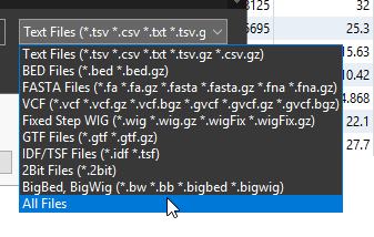
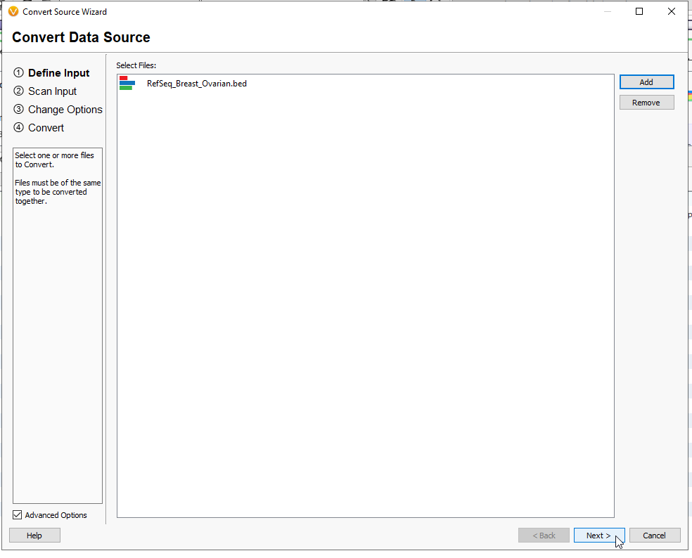
First hit the Add button, and find the BED file that you previously downloaded. While searching for it, remember to change the drop down from Text File to either BED Files or All Files (Figure 10). Hit Open.

The BED file will appear with the red, blue, and green stripes, indicating an interval track (Figure 11). Hit Next.

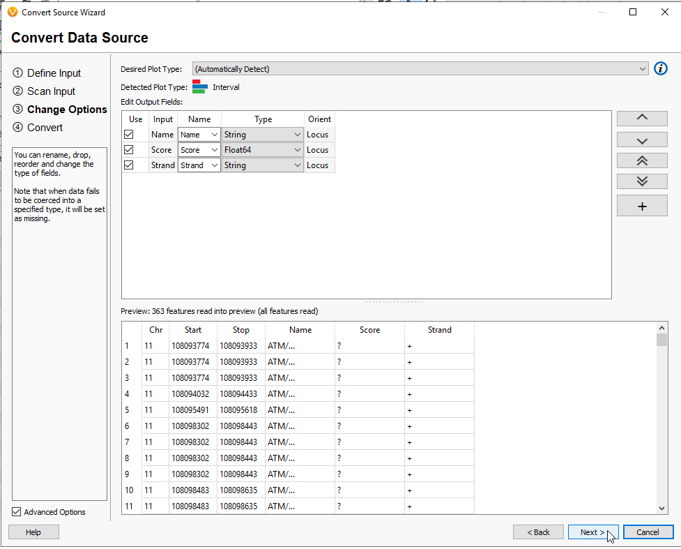
This page will show the default fields, along with the plot type which is automatically recognized as Interval (Figure 12). You may add more fields with the + Button, but for the goal of running Coverage Statistics, this is not needed. Hit Next.

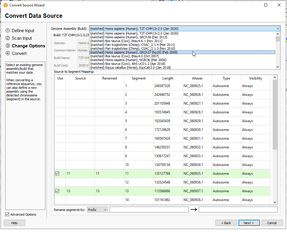
This next page will have you designate the Genome Assembly Build (Figure 13). I am working with GRCh37. If you exported only a reduced list of genes, and not all of the coding regions, you will likely notice that not all of the chromosomes are being indicated in this view. This is because our small gene track has genes on Chromosome 11, 13, etc.. Hit Next.

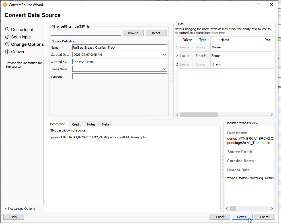
You are then able to give this track a name, and any notes related to the tracks purpose, or who curated it (Figure 14). When you are ready, hit Next.

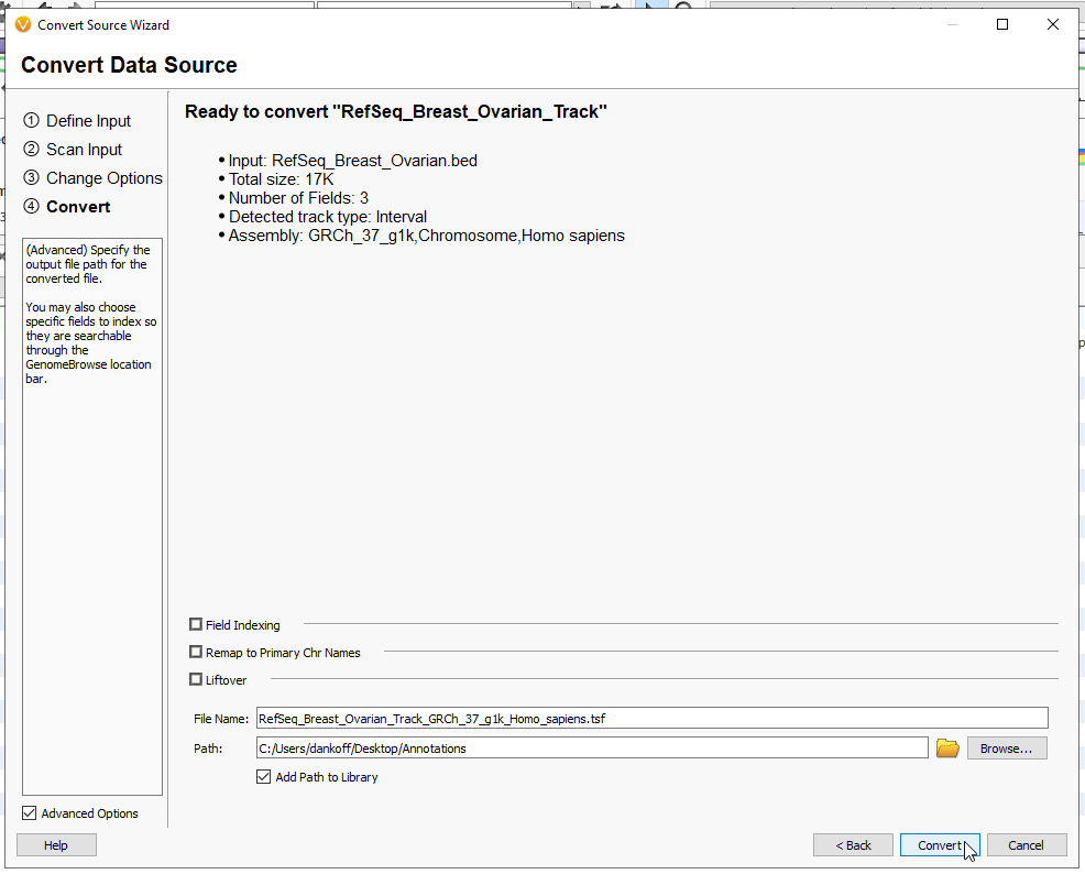
This last page will summarize the inputs so far, such as the track type and the assembly (Figure 15). When the settings look good, give your file a name, and decide where you want the tsf to download. By default, these tracks will go into the annotations folder. By adding path to the library, it will automatically show up in the Annotations Folder (from the Annotations folder, you can also ‘refresh’ the contents to bring in the new interval track). Now hit Convert, and the file will render as a tsf. You may close the window when it has completed converting.

Step 4: Running Coverage Statistics

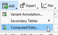
After associating your alignment file and creating a converted interval track file, you are ready to run Coverage Statistics! Go to Add > Computed Data (Figure 16).

Pick the Target Region Coverage option (Figure 17). Here you will also see the Binned Region Coverage. This option is more appropriate when looking at whole genome coverage. Our Target Region Coverage is useful for Gene Panels and WES samples. The Targeted Region Coverage is going to bring in many fields and different tables. There will be a new Coverage Regions Table that will define coverage at specified depths, there will be a Variants by Region table, and summary statistics fields in the Sample Table.

To run the Coverage Statistics Algorithm (Targeted Region Coverage), select the track previously created (Figure 18). If you want to add additional depth thresholds for reporting, you can add them below. You also have the ability to collapse overlapping regions defined in your BED file to single regions, and to count only proper flagged (0x02) reads. Including this flag signifies only the use of reads in which both ends of the read were properly mapped and they were mapped within a reasonable distance given the expected distance provided to the alignment software.

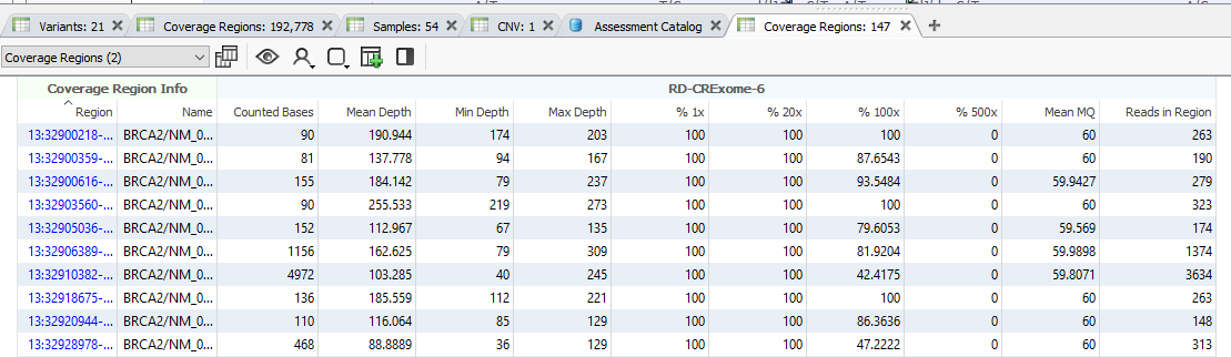
And with that, the Coverage Regions will start to calculate (Figure 19). Depending on the size of the project, the number of regions, and the RAM on your machine, this may run quickly, or it may take some time. Feel free to grab a cup of coffee and watch the green progress bar think. Once this has finished, you will have a complete Coverage Regions tab, with additional fields in Samples and Variants tables.

Make sure to go back to Add > Computed Data, and drop down the table type to Coverage Regions to view a number of algorithms only available for coverage data. These coverage statistics can provide invaluable data for reporting, or if you plan on using the VarSeq CNV caller.

If you’re interested in seeing the software in action or have any questions about the steps outlined in this guide, reach out to support@goldenhelix.com and request a demo. One of our knowledgeable FAS members will be happy to walk you through the software during a training call. Have a great Valentine’s Day, and happy BEDing!