Pruning your data based on Linkage Disequilibrium (LD) values is an important quality assurance step for GWAS analysis. In particular, some tests such as Identity by Descent Estimation (IBD), Inbreeding Coefficient Estimation (f) and Principal Component Analysis (PCA) will obtain better results if the markers used are not in linkage disequilibrium with each other. Therefore, Golden Helix’s SVS provides the LD Pruning feature to inactivate (prune) markers that are in LD with other markers. This allows you to perform your test directly on a set of activated markers with low LD compared to each other.

The LD Pruning method can be launched from any genotype spreadsheet in SVS by going to Genotype > Quality Assurance and Utilities > LD Pruning. For this method all pairs of markers within a moving window are compared with each other to measure their pairwise LD. If any pair of markers within the window are in LD greater than the specified threshold, the first marker in the pair will be inactivated (pruned).

The options for pruning your markers are specified in the options dialog with the default options being the most common choices for basic pruning of the data. However, if your marker data is dense in some areas or you see large blocks of moderately high LD in other areas that you would like reduced, changing these default options may improve your results.

We will take a look at 54 markers in the region of the SLC6A3 gene to see how the different pruning options affect the results. LD was computed on markers from the CEU population provided from HapMap Phase3 genotypes obtained from the NCBI FTP site.

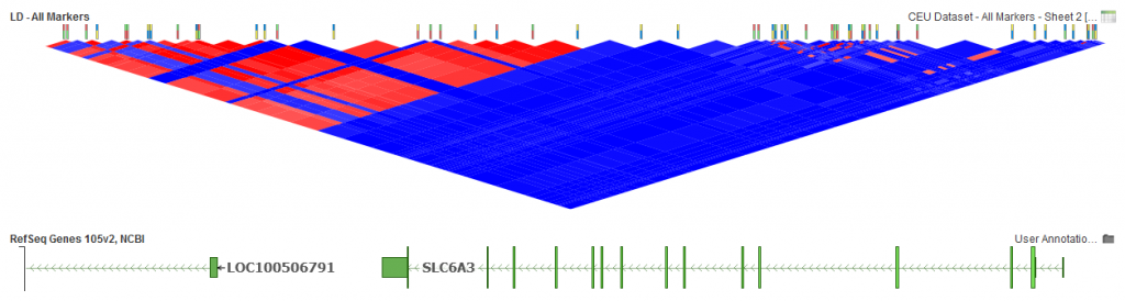
Fig. 1. LD for all 54 markers.

Using the default options (Fig. 2) available on the LD Pruning dialog inactivates 33 markers and leaves 21 markers for further analysis active.

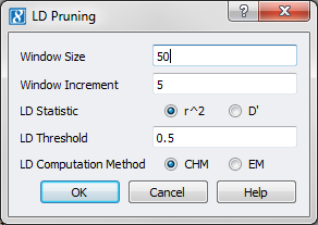
Fig.2. Default LD Options

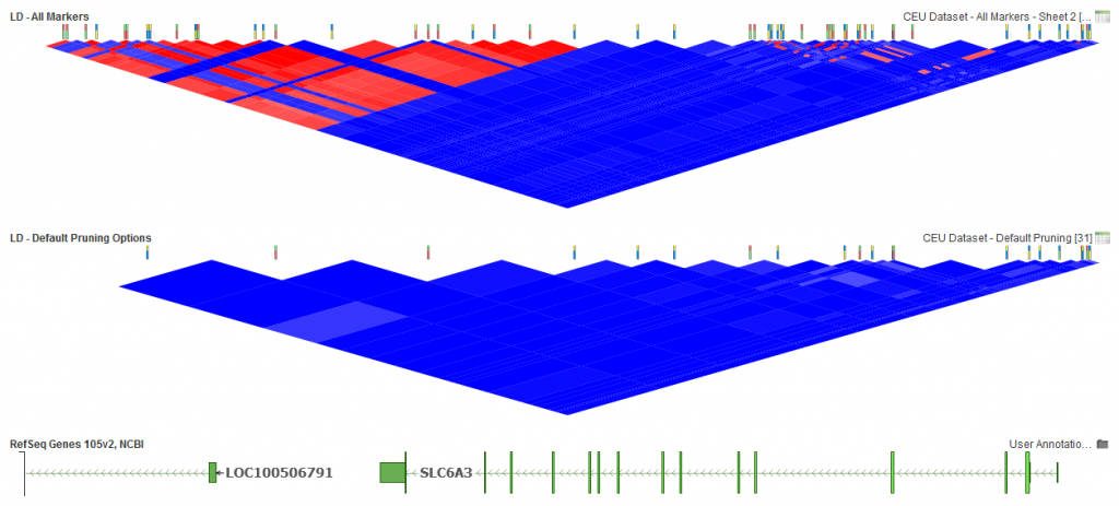
Fig.3. 21 activated markers left with default options.

We will now take a look at adjusting LD Threshold, window increment and window size to see how these options can affect the results for this set of markers.

The LD Threshold option is the determining factor in whether there will be pruning between pairs of markers. If the pairwise LD value is greater than the threshold, then pruning will happen. However, if it is less, both markers will remain active. So in general, the lower the selected LD Threshold, the more markers will be pruned. Similarly, the higher the threshold, the fewer markers pruned. Below is how that looks for this dataset if thresholds of 0.25 and 0.8 are chosen.

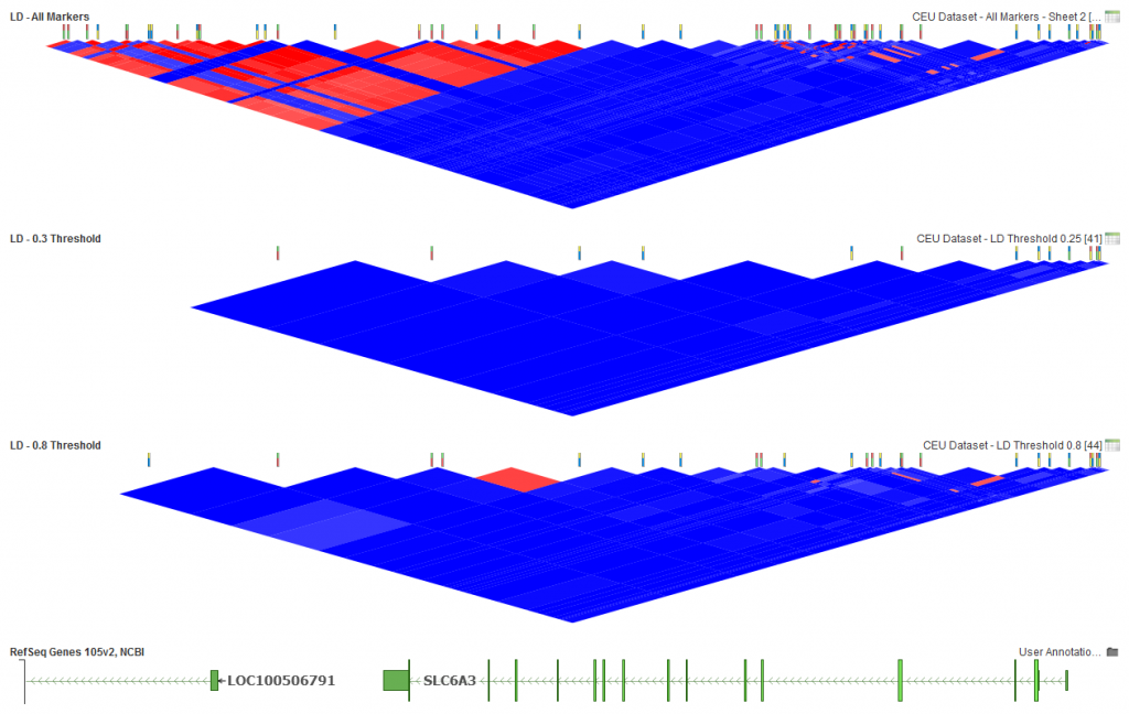
Fig.4. LD Threshold of 0.25, 13 active markers and LD Threshold of 0.8, 25 markers activate.

In the middle plot above (Fig.4), you can see that all red blocks have been removed, leaving only those markers with low pairwise LD in the dataset. In the bottom plot, you can see some light red areas have been left using the selected options. So if you are looking to remove any indication of LD between markers, the lower the threshold the better, but if some level of LD is acceptable then a higher threshold can be selected.

Next, let’s take a look at how window size can affect the results.

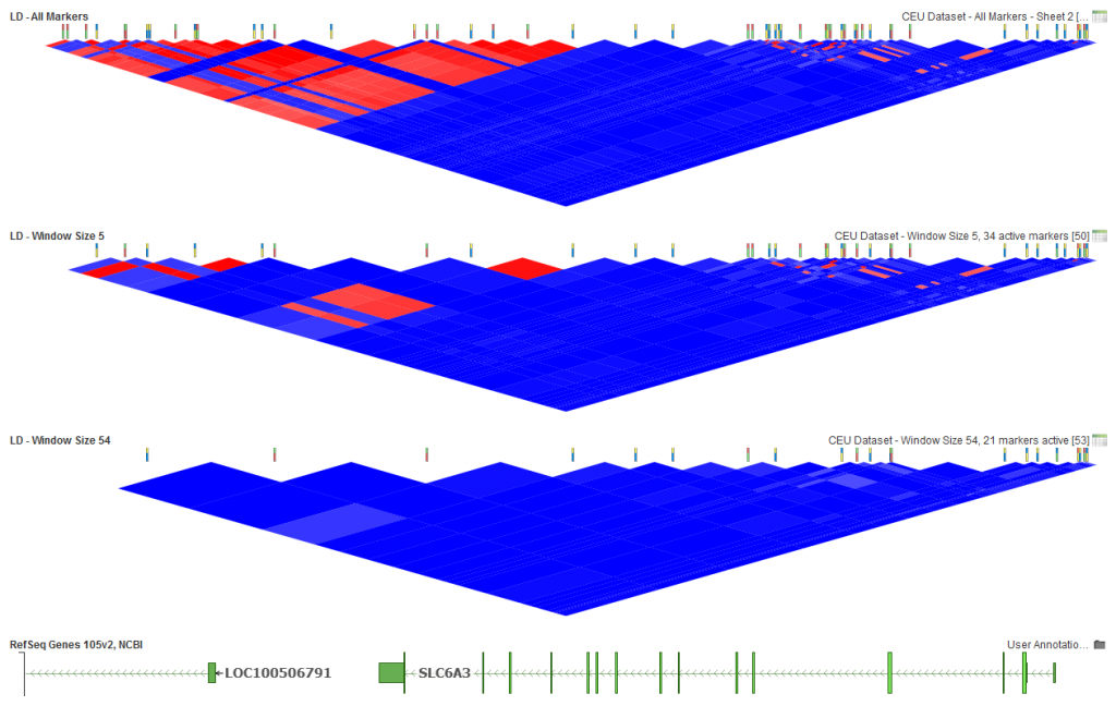
Fig.5. Window size of 5 markers, 34 active markers and Window Size of 54, 21 active markers.

With this dataset, an extremely low window size (5) will make it so LD between markers that may still be close based on base pair distance are not even compared. You can see in the middle plot above that the lower portion of the triangle still has some red to indicate the existence of markers in high LD. With a large dataset, you will also find that increasing the window size can speed up the algorithm as less pairwise comparisons are made for the analysis.

For the bottom plot above (Fig.5), 54 was selected as the window size. Since there are 54 markers in this dataset, that means that all pairs of markers were compared. For larger datasets, memory limitations will not allow for this many comparisons so you will need to pick a reasonably sized window that will work with the memory limitations on your system.

Lastly, let’s take a look at window increment options in the analysis. For this dataset, we will also need to lower the default options for window size to 10. The default size of 50 would include nearly all the markers in this sample dataset so you would only see a difference when the window size is low enough to be effective.

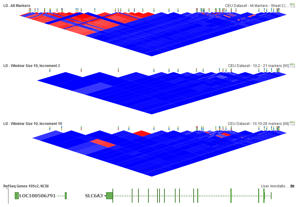
Fig.6. Window Increment 2, 21 markers active and Window Increment of 10, 28 markers active

With a Window Size of 10 for this dataset, a low window increment will provide enough of a pairwise comparison to remove those markers in high LD. However, if an increment value equal to the size of the window is picked, this will result in adjacent markers at the boundaries of the windows not being compared. This leaves some markers active that could be in high LD. If you selected an increment larger than the window size, then large groups of markers could be skipped. So window increment size by itself does not have much effect and should just be less than the window size to have the best performance.

Each of these options together or separately can be adjusted to get the best results for your data and analysis needs. Please contact support@goldenehelix.com if you have any questions or need assistance with your analysis.