While VarSeq comes with a number of starter workflows that are stored as templates, customers also have the option of creating filter chains from scratch; analyzing a single exome may require you to do exactly that. In this blog, I’ll go through analyzing a single exome and generating a list of variants for further study.
After importing the variant data into VarSeq, you will notice a full variant table and an empty filter chain. Before adding annotation data, the fields from the VCF file can be used for quality assurance. First, I used the Read Depth and Genotype Quality fields with minimum thresholds of 10 and 20 respectively, highlighting those variants above these thresholds.
After these standard steps, there is a lot of flexibility as to what Annotation Sources or Computations to add to the dataset next. That’s part of the fun with using VarSeq! You may want to start by computing the Zygosity State of the variants in the dataset. The zygosity state feature is helpful if you are aware of the type of variant you are looking for. Homozygous would be relevant for a recessive phenotype and removing reference alleles is beneficial if multiple samples were called together in secondary analysis.
There are additional options for narrowing down the type of variants you are interested in, and there are also options for filtering based on a gene list or genomic region, for example.
This particular individual presented clinically with mental retardation and facial abnormalities. Based on the family information, it seems to be caused by a rare variant, so next the common variants found in the population can be removed. First, common variants found in dbSNP were removed. Then using population level minor allele frequency data from NHLBI and ExAC databases, variants higher than a 1% frequency were removed using the African American population information as that is the ethnicity of the patient, Figure 1.
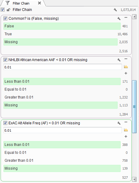
Figure 1. Set of filters finding rare variants.
After removing the common variants, there is a lot of flexibility as to the Annotations Sources included next and how to continue filtering the exome variants. In this case, we know the variant has a severe phenotype so using a gene track such as RefSeq to gain sequence ontology information would be beneficial. The sequence ontology information can be used directly or when annotating against a gene track, the Effect of each sequence ontology term is listed. This is simplified into Loss of Function (LoF), Missense or Other (definitions seen below in Figure 2).
In this case, the Effect simplification was used and LoF and Missense variants were kept. Next, the Functional Predictions annotation source was implemented. This track includes the pre-computed functional predictions for five different algorithms identifying if variants are damaging or tolerated: SIFT, Polyphen2, MutationTaster, MutationAssesor and FATHMM. VarSeq tabulates these sources into the number of algorithms that consider a variant damaging or tolerated, so you can select how many out of those five consider it damaging. Also, each of the different algorithms’ results can be used for filtering if you have a favorite algorithm in mind!
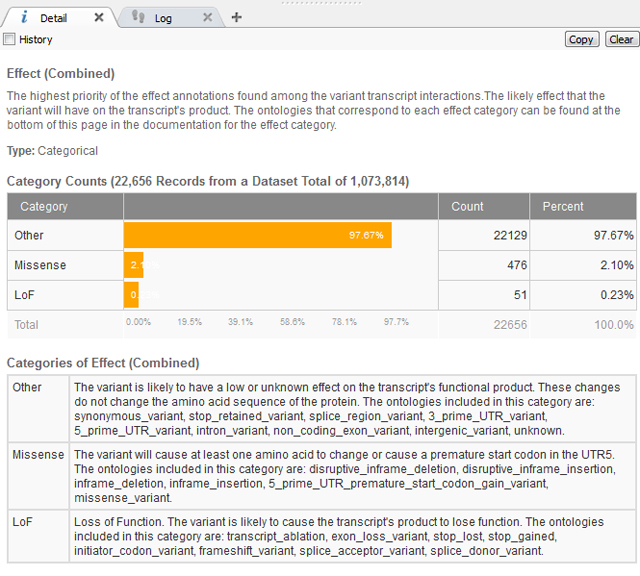
Figure 2. Definitions of “Effect” information for Gene Track from RefSeq105v2.
After starting with over 1 million variants, we have filtered down to 106 that could potentially be disease causing. A final algorithm we can implement to narrow these down even further is PhoRank. This computation is based off the Phevor algorithm and searches through the HPO and GO biomedical ontology databases finding genes that are correlated with the set of phenotypes associated with the individual. In this case, this individual’s phenotypes are mental retardation and microcephaly. However, mental retardation is not a term found from either database, but this phenotype can also be called neurodevelopmental delay, which is a term found in GO and HPO. Using these two search terms the results show a Gene Rank, Gene Score and Path, described below.
- Gene Rank: Percentile rank of the specific gene.
- GeneScore: The score of the gene computed by the ontology propagation algorithm.
- Path: A shortest path from the gene to one of the specified phenotypes (there may be many paths to the phenotypes).
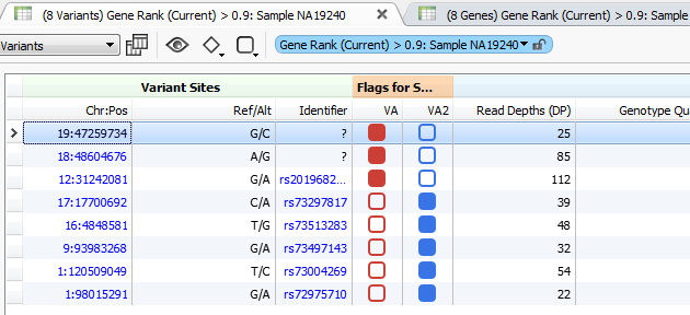
Figure 3. Variant Tags in VarSeq
The higher the Gene Rank, the more correlated the gene is with the phenotypes entered and the shorter the path through the databases. In this case, the Gene Rank score was used with variants falling in the 90th percentile, which leaves eight variants to consider. Now that there are only eight variants to consider, this information can be passed on to a colleague or the clinician for review. That’s where VSReports comes in! I’ve created two sets of variants based on their entry in ClinVar; three variants have been noted in ClinVar and five have not, Figure 3. This tagging feature was used to separate these two sets of variants which can then be included in a report, Figure 4. Finally, after entering in the desired information for each variant the report can be created and exported from VarSeq in a PDF.
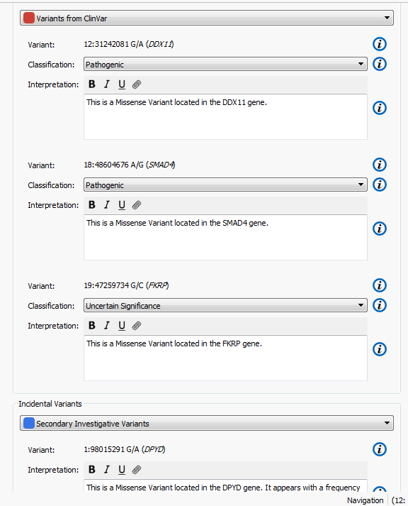
Figure 4. Set up for creating a report in VSReports including two variant sets.
VarSeq was designed to provide researchers and clinicians with an easy-to-use software that has a user friendly GUI for variant annotating and filtering. The example workflow in this blog just scratches the surface on the annotations and computations available in VarSeq. If you’re interested in trying out VarSeq for your research, please contact support@goldenhelix.com!