New SVS Meta-Analysis Example Project

The latest version of the GWAS E-book featured a chapter on Meta-Analysis. We are pleased to make the project used in this chapter available as an example project for SVS (SNP & Variation Suite). This blog post will walk you through the analysis steps used in the example project. This information is also contained in the User Notes view in the project navigator for all project nodes that have the “N” tag to the left of the node name.

You can follow along either with a licensed version of SVS or with the SVS Viewer. The SVS Viewer is available for free and allows you to view existing projects (spreadsheets and non-genomic plots) and visualize data in genomic contexts using GenomeBrowse.

After downloading the SVS Viewer, download the Example Project by clicking on the Example Projects link or click on the Download menu and select Example Projects.

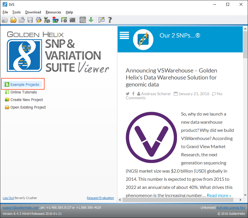
Fig. 1. SVS Viewer Welcome Screen

Select the Meta-Analysis Example Project – Complete project from the list.

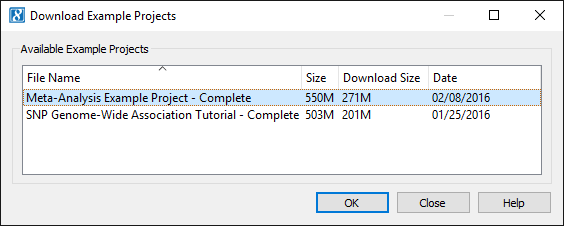
Fig. 2. Selecting the example project to download

The downloaded example project will automatically open after the download is complete. If you are not familiar with the SVS project interface, this project navigator view will contain three areas: the Navigator Window Nodes on the left, the Node Change Log on the upper right and the User Notes on the lower right. The User Notes can be edited and modified by the user with a licensed version of SVS to capture important information about settings and parameters used as well as interesting findings. In this case, we have detailed all of the steps taken for the meta-analysis project for those using the SVS Viewer to be able to follow along.

Note: The Meta-Analysis methods implemented in SVS are documented in our manual.

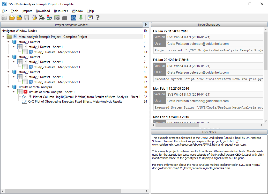
Fig. 3. Meta-Analysis Example Project – Complete project navigator

This example project contains results from three different association tests. The datasets used for the association tests were subsets of the Marshall Autism GEO dataset with slight modifications made to the genotypes to display a signal in the SRPK1 gene.

Four nodes in this project are color coded, the three blue nodes are the three original study results spreadsheets, the red node is the final Meta-Analysis results from combining the three blue nodes.

Click on the red node “Results of Meta-Analysis – Sheet 1” and you will see details about the parameters used in the User Notes.

With a licensed version of SVS you can recreate the Meta-Analysis results. To do this, you would go to Tools > Perform Meta-Analysis and select the three nodes with the blue tags (nodes 13, 15 and 18). The defaults for the other parameters in the initial dialog were used, see Fig. 4.

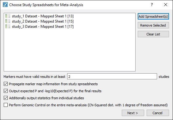
Fig. 4. Select the study spreadsheets for Meta-Analysis

After setting these parameters, Next > was clicked to open the options for each study. Setting the options for the first study sets the defaults for the subsequent studies to make it easier if the data was generated from the same source. The defaults can be changed if the fields are not named the same.

In this case, Sample-Sized based Inputs were used. However, the data for Inverse-Variance-Based Inputs is included in these spreadsheets and can be computed with a licensed version of SVS.

Fig. 5. shows the study options that were used for “study_1” (node 13):

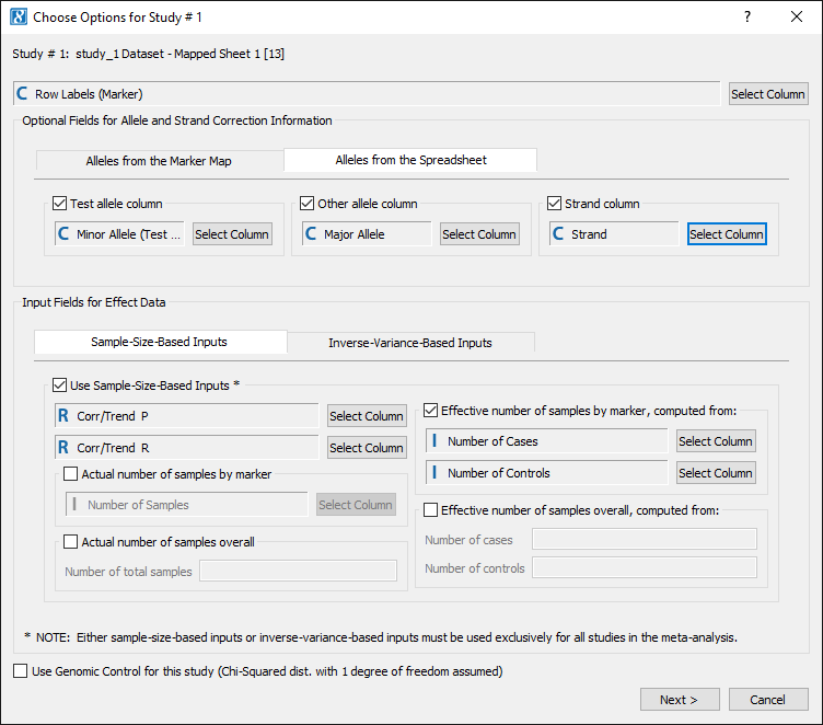
Fig. 5. study_1 Parameters for Meta-Analysis

As you can see in Fig. 6. there are fewer parameters for “study_2” (node 15), the available parameters are set by the options selected for the first study.

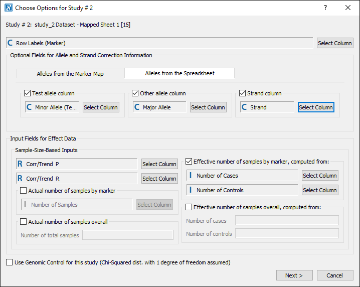
Fig. 6. “study_2” and Subsequent Study Parameters are Restricted based on “study_1” Selections

The result of the Meta-Analysis is a spreadsheet containing results for both a fixed-effects and random-effects meta-analysis models. Based on our choices, this spreadsheet also contains the relevant per-study input.

Fig. 7. Meta-Analysis Results Spreadsheet

From this spreadsheet you can plot a Manhattan plot of the -log10(Overall P-Value) column. In this case, the fixed-effects model is the appropriate model. With the SVS Viewer or a licensed version of SVS you can recreate figures 17 and 18 from the GWAS E-Book. To create your own Manhattan plot go to GenomeBrowse > Numeric Value Plot and select “-log10(Overall P-Value)”.

To add in the original -log10 P-values from the three studies, from GenomeBrowse click on the “Add” button in the upper left-hand corner, and then select “Project”. Click on “study_1 Dataset — Mapped Sheet 1” ( node 13 ) then click “Plot & Close”.

Next, click on the Corr/Trend -log10 P parent node in the graph tree on the left and click on the Add tab. Click on “Add Item(s)” with “Project” selected, click on “study_2 Dataset — Mapped Sheet 1” ( node 15 ) and select “Corr/Trend -log10 P”. Do the same for “study_3”, then click “Plot & Close”.

This will create two plot items in the same graph with the same color. To recolor the plots, click on the “Style” tab for the parent node (graph node) and click on “Apply” next to “Restyle: [ From Current ]”.

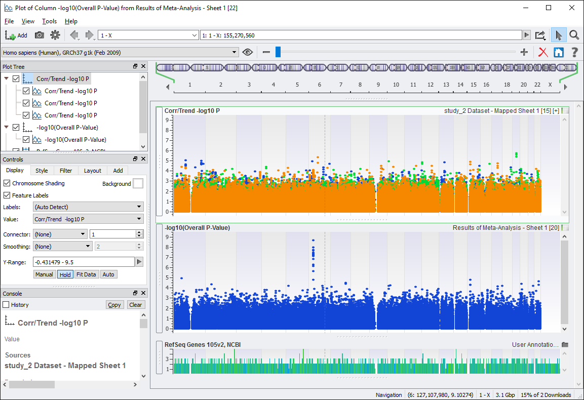
Fig. 8. Meta-Analysis Manhattan Plot of the Overall P-value Compared to the Individual P-Values (Fig 17 in GWAS E-book)

You can scroll in and out to zoom in on the peak in Chromosome 6, or you can type in the gene name “SRPK1” into the location bar, or enter in this zoom region: 6: 35,800,811 – 35,888,957.

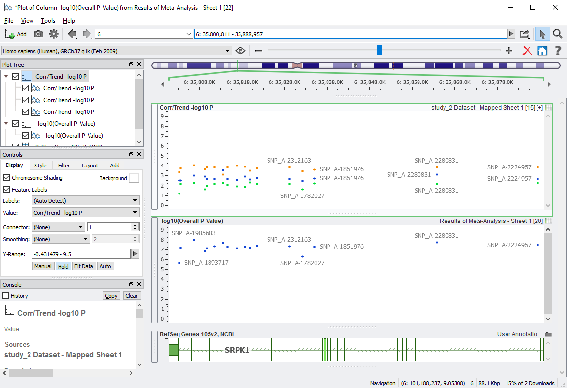
Fig. 9. Meta-Analysis Results Zoomed to the SRPK1 Gene (Fig 18 in the GWAS E-book)

To further examine the most significant results a Meta-Analysis Forest plot is useful. This can be done with a licensed version of SVS from the Plot menu. With the SVS Viewer, the forest plot for the top result has been created and is included in the example project.

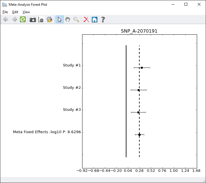
Fig 10. Forest Plot for the Most Significant SRPK1 SNP

To explore this project, including a Q-Q plot not mentioned in this blog post, you can download the SVS Viewer here. If you have any questions, please feel free to contact us at support@goldenhelix.com.