Solving the Eigenvalue Decomposition Problem for Large Sample Sizes
Since our introduction of the mixed model methods in SVS, along with GBLUP, we have been very pleased to see it used by a number of customers working with human and agri-genomic data. As these customers have grown their genomics programs, the number of samples they have for a given analysis has been growing, and at times exponentially!
Up to this point, scaling these algorithms has just been about doing the analysis on an adequately large computer (specifically one with sufficient memory to hold these large N2 matrices, where N is the number of samples).
But now, for some customers working in consortium or national scale breeding programs, the number of samples are reach 100,000 or more. The squared nature of these matrices exceed the fundamental limits to what operating systems allow for contiguous chunks of memory, even if you do have the hundreds of gigabytes of physical RAM available.
These limitations have been reached in SVS by the matrix multiplication operations required by the Efficient Mixed Model Analysis eXpedited (EMMAX) [Segura2012, Vilhjalmsson2012, Kang2010, Kang2008] and Genomic Best Linear Unbiased Prediction (GBLUP) [VanRaden2008, Taylor2013] algorithms.
So if we can’t throw more compute power at the problem then we need to find a way to adapt the algorithms to work with the limits imposed by operating systems.
Now this isn’t a problem we need to solve by inventing completely new algorithms, we just need to solve the algorithms by leveraging different existing mathematical methods to do these matrix math operations on large dimensional datasets in an approximation of the expensive exact methods.
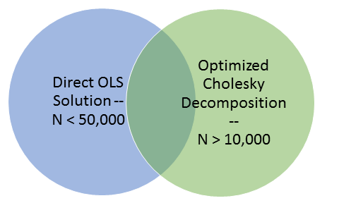
Fig 1: Venn Diagram demonstrating the overlapping sample numbers that can be used to validate results between the two solution approaches
We can partition the solving of these problems into two overlapping groups. The first group contains datasets with fewer than fifty thousand (50,000) samples, the second group contains datasets with more than ten thousand (10,000) samples. Fortunately, this problem is not affected by the number of markers. Because of this overlap in the problem space we can use the approximate answers for datasets with more than 10,000 samples to gauge the correctness of the results for datasets with larger than 50,000 markers.
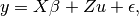
The standard direct method used to solve GBLUP or EMMAX regression equations is as follows:
- Find the generalized least squares (GLS) solution to the mixed linear model equation
 by finding a matrix B such that:
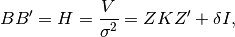 where the variance of
  is
is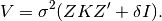
NOTE: To solve both the equations for EMMAX and GBLUP using ordinary least squares (OLS) a B-1 matrix is required. The Cholesky decomposition of H is one way to obtain such a matrix B.
- Determine a delta for the intercept-only case.
- Determine a delta for the covariates case, if non-intercept covariates are used.
So far, these have been accomplished by finding the eigenvectors/eigenvalues of the kinship matrix K (for “B inverse”) and S(K + I)S (for finding delta).
Finding eigenvectors and eigenvalues of a square matrix normally reduces to
- The computationally intensive part, where it is computing the “interesting” eigenvectors that have the higher eigenvalues.
- A continuation of the computationally intensive part, but the eigenvalues are getting lower and for some purposes we may be able to neglect them if they are not too different from their minimum possible value.
- An “easy part”, where all the eigenvalues are at their minimum possible value and execution is fast(er). Happens if the original genotypic data from which K was created had more samples than markers. Also happens sometimes with collinear genotypic data.
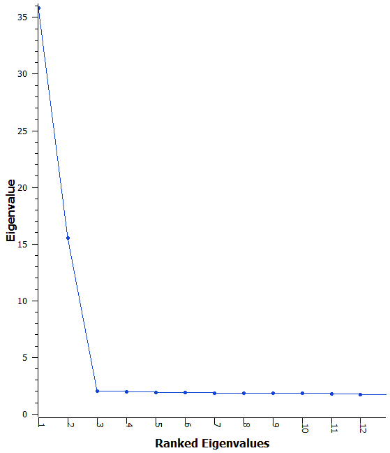
Fig. 2. Scree Plot of the first 12 Eigenvalues demonstrating that after the first few eigenvalues the difference between values is quite small
To solve this we are using mathematics to remove the need for finding the S(K + I)S eigenvectors for the minimum eigenvalue of 1. To find the “B inverse” matrix a Cholesky decomposition (specifically the Cholesky-Crout algorithm [Press2007]) of the kinship matrix K (or of (K + δI) for stability). When the algorithms call for “Multiply by B inverse” this would be done through forward substitution for each vector being multiplied.
As we work on solving this problem we have to balance the need for handling the large numbers of samples with reasonable expectations of computing resources available and being reasonably fast. One of our first attempts on analyzing 90K samples ran for a week after finishing the kinship matrix computation before filling the 10 TB hard drive with temporary datasets and crashing due to running out of disk space! Our final version will not store large temporary matrices longer than necessary to prevent over consumption of hard disk space.
Before releasing these methods to the public we will be giving early access to a limited number of beta testers who have datasets of this size ready and waiting for analysis. If you want to be included in this early access period, please let us know.
Our first release will include large N versions of GBLUP, Computing the Genomic Relationship Matrix, and Mixed Linear Model Analysis. Future releases will include making these methods available for Bayes C/C-Pi and Principal Component Analysis (PCA).
References:
Kang HM, et al (2008). ‘Efficient control of population structure in model organism association mapping’, Genetics, 178, 1709–1723.
Kang HM, et al (2010). ‘Variance component model to account for sample structure in genome-wide association studies’, Nature Genetics 42, 348–354.
Press, William H. (2007). Numerical Recipes 3rd Edition: The Art of Scientific Computing. Cambridge University Press. pp. 50–52. ISBN 9780521880688.
Segura V, Vihjálmsson BJ, Platt A, Korte A, Seren Ü, et al. (2012) ‘An efficient multi-locus mixed-model approach for genome-wide association studies in structured populations’, Nature Genetics, 44, 825–830.
Taylor, J.F. (2013) ‘Implementation and accuracy of genomic selection’, Aquaculture, http://dx.doi.org/10.1016/j.aquaculture.2013.02.017
VanRaden, P.M. (2008) ‘Efficient Methods to Compute Genomic Predictions’, J. Dairy Sci, 91, pp. 4414–4423.
Vilhjalmsson B (2012) ‘mixmogam’ https://github.com/bvilhjal/mixmogam. Commit a40f3e2c95.
Be glad to give you improved scripts a run on our larger cattle dataset. Currently have 520,000 animals (>20 breeds) most (~320,000) with ~50k genotypes. Also can you look into having the FImpute input scripts handle larger datasets? For the 320k aniamls with 50k genotypes I need to filter groups of ~35k out and write their FImpute scripts separately. Also can you work on if PCA analaysis can be done with larger datasets like mine?
FYI your GRM can do ~80,000 animals for 7k markers (did this last week).
Matt