The support team at Golden Helix is always here to help with your SVS and VarSeq needs. Often, we receive some excellent questions that should be shared with the rest of our users. This blog will answer some common questions we’ve been seeing lately regarding VarSeq CNV.
- I’ve noticed there is a version 2 of the CNV caller on Targeted Regions Algorithm, how has this changed from version 1 and does this alter my workflow?
Our development team works extremely hard to develop new features and improve existing algorithms. As Gabe Rudy had mentioned in his blog post, we have been benchmarking against CMA validated clinical samples from PreventionGenetics and other external collaborators to improve the sensitivity and precision of the algorithm. The development team rolled these improvements into the latest 1.4.5 CNV target caller to provide excellent CNV calls on exome and gene panel data.
The question remains, do these improvements alter my existing workflow? If you are interested in calling CNVs on your gene panels or exomes, we suggest that you first run our Loss of Heterozygosity (LOH) caller which looks at the Variant Allele Frequency (VAF) of the imported variants.
The LoH has been updated in 1.4.5 with improved sensitivity, as well as a model for calling Triploid events. The CNV algorithm will pick this up as input, and through improved normalization make better CNV calls and report Copy Neutral LOH events.
Is there a way tell if you have sample contamination in VarSeq?
If you suspect that you have some level of sample contamination you could examine the variant allele frequency (VAF) calculated for homozygous variants. The VAF field is not always provided directly in the VCF data but don’t worry, VarSeq will automatically calculate the frequency using the provided allelic depth fields in the file. For homozygous variants, we would expect a VAF to be 1.
For example, in the CNV analysis below we have a female sample with a reported XXY karyotype.
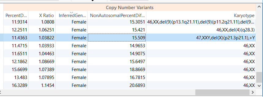
Figure 1. Copy Number Table Output. Note the Karyotype of the third sample.
Indeed when we plot this CNV in GenomeBrowse along with the VAF field, we can see some reads partially mapped to the Y chromosome…..head scratching ensues……What if this was a female sample who happened to be pregnant with a boy? Could we be picking up some fragments of the Y chromosome in the bloodstream when sequencing?….How cool would that be!

Figure 2. The sample plotted in GenomeBrowse with CNV State, Variant Allele Frequency, Mean Depth and RefSeq genes.
To check if this scenario is plausible, I can create a couple of filter cards on the genotype (GT) field and the VAF field in the variant table to examine the ratio of homozygous variants that have VAF of less than 0.98. A higher proportion of variants across the genome that have a lower VAF for homozygous variants would likely indicate some sample contamination.
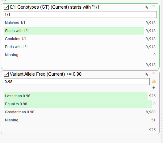
Figure 3. Filtering on Genotype (GT) and VAF field.
In this example, out of the 9,918 homozygous variants, 925 had a VAF of less than 0.98. So 925/9918 = 9.33%. That seems a bit high and examining other samples in the data set I find that percentages to be much lower (around 1%). After reviewing the evidence here, I concluded its very likely that there was some sample contamination from a male for this female sample.
Can you exclude low coverage regions from your CNV analysis?
An excellent question. After running the Targeted Region Coverage algorithm, some users have run into instances where the majority of their samples have large regions with very low coverage. If you are conducting CNV analysis on gene panel data, you may want to exclude these regions.
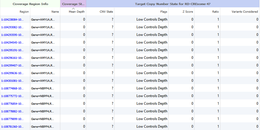
Figure 4. Coverage Region Table regions exhibiting no mapped reads.
One way to do this is to query the Mean Depth column in the Coverage Regions table and enter >=100.
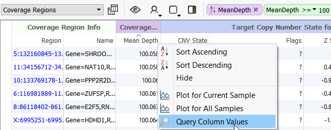
Figure 5. Sorting the Coverage Table.
Then export the resulting list to excel to edit.
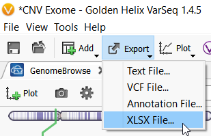
Figure 6. Exporting a table to Excel.
Your BED or interval track is used to define the regions that coverage (and ultimately CNVs) gets computed over. This interval file minimally needs a chromosome, start and stop position.
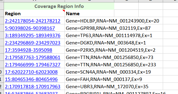
Figure 7. Coverage Regions Table exported in Excel.
With a little editing I can create a chromosome, start, stop and optional name column in excel and save this as a comma delimited (.CSV) file to import back into VarSeq using the Annotation Convert Source Wizard.
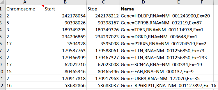
Figure 8. Edited BED file ready to import into VarSeq to be used as an interval track.
Now that I have my new BED file into the software, I am ready to re-run the Targeted Region Coverage Algorithm and call CNVs.
How can I determine if the samples best match my reference sample set?
Before diving in to evaluate each CNV event, its always a good idea to open a new Samples table in VarSeq. This sample table will contain coverage and useful CNV sample summary information.
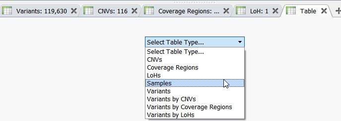
Figure 9. Opening a new Samples Table.
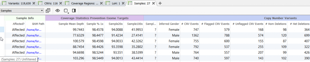
Figure 10. Sample Table Containing Summary Coverage and CNV Information.
Two columns of interest are the Percent Difference and Reference Samples columns.
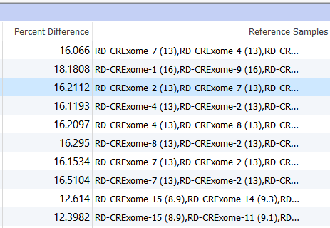
Figure 11. Percent Difference and Reference Samples Column In the Samples Table.
The Percent Difference column states the average percent difference between a given sample and the matched controls for autosomal regions. We find that samples perform optimally if the average percent difference is less than 20% for a given sample. The Reference Samples column will give you a more detailed comparison. This column will list each sample used in the reference sample set and record the average percent difference in parenthesis. By default, this list is sorted in ascending order. So the samples with the best match are listed first and the poorest samples listed last. You can optionally right-click on this column header and copy and paste this list in a text editor to examine all samples chosen. If you find that a given sample is a consistently a poor match you can open your reference sample folder and remove the sample from your reference set.
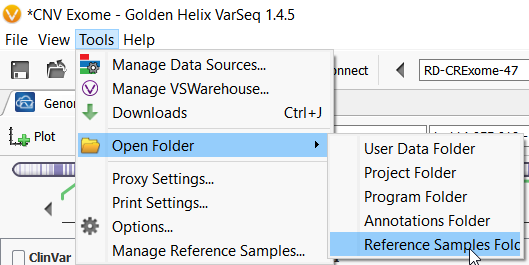
Figure 12. Opening the Reference Samples Folder.
I understand that the CNV caller on Binned Regions was developed to call CNVs from low and ultra-low read depth Whole Genome Sequencing (WGS) data. If I have WGS data with higher coverage, can I use the CNV Caller on Target Regions algorithm?
Another excellent question! Lets first briefly review the two algorithms and discuss some of their distinctions. The CNV caller on Target Regions algorithm was originally developed for gene panels and its use was expanded to call both large (10 kb +) and small CNV (1000bp) events from exome data as well. We have found the algorithm consistency called all CNVs in our validation sets when the coverage is close to 100x for each targeted region. Several users have reported to us that they have had excellent results when evaluating the CNV algorithm on their validated sets with much lower coverage.
Data from WGS typically does not yet rise into 100x range across target regions, so our development team produced another algorithm that can call large cytogenetic events from WGS data, with minimal coverage requirements (~0.02x).
Since the CNV caller on Binned Regions algorithm has been released, many users have asked us if ~60x coverage is sufficient to run the CNV caller on Targeted Region algorithm with WGS data. From some of our higher coverage WGS samples (~60x), we have found the algorithm can still provide great CNV calls, so I would give it a try. With that in mind, mean depth over a targeted region is just one factor in evaluating the performance of the algorithm.
Ultimately, Gabe Rudy said it best, “No algorithm developed purely on the theory of how data should look survives the first contact with the reality of the unpredictable nature of real-world data.”
Can you detect copy-neutral and triploid LOH events?
Yes. Since the release of VarSeq 1.4.5, the development team has updated the LOH caller. The new Triploid (Trisomy) state is called when the Hidden Markov Model is able to clearly detect a likely duplication purely based on the distribution of the Variant Allele Frequency. In the example below you can see the CNV calling algorithm call a duplication (see the elevated Z-score!) with VAF clearly forming a pattern around this region. The VAF in triploid regions will cluster around 0.2-0.4 and 0.6-0.8 forming a distinctive pattern when plotted in GenomeBrowse.
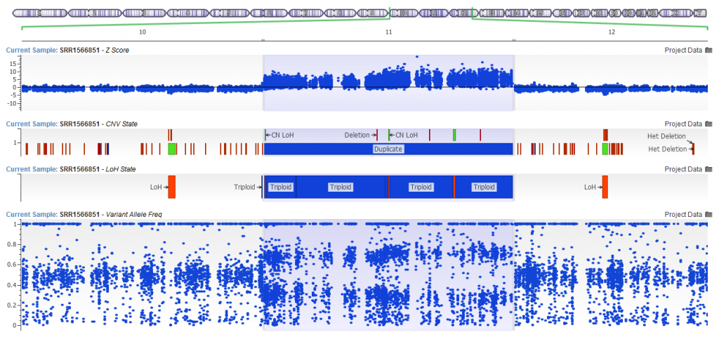
Figure 13. Trisomic Calls from the LOH Algorithm.
LOH events are a common occurrence in cancer, where it indicates the absence of a functional tumor suppressor gene in the region. Copy neutral LOH events are denoted in green when plotted in GenomeBrowse. In the image below you can see the vast majority of VAF values in this region, do not differ from one. The variants that do differentiate from 1 in this multi-gene region have low mapping quality scores.
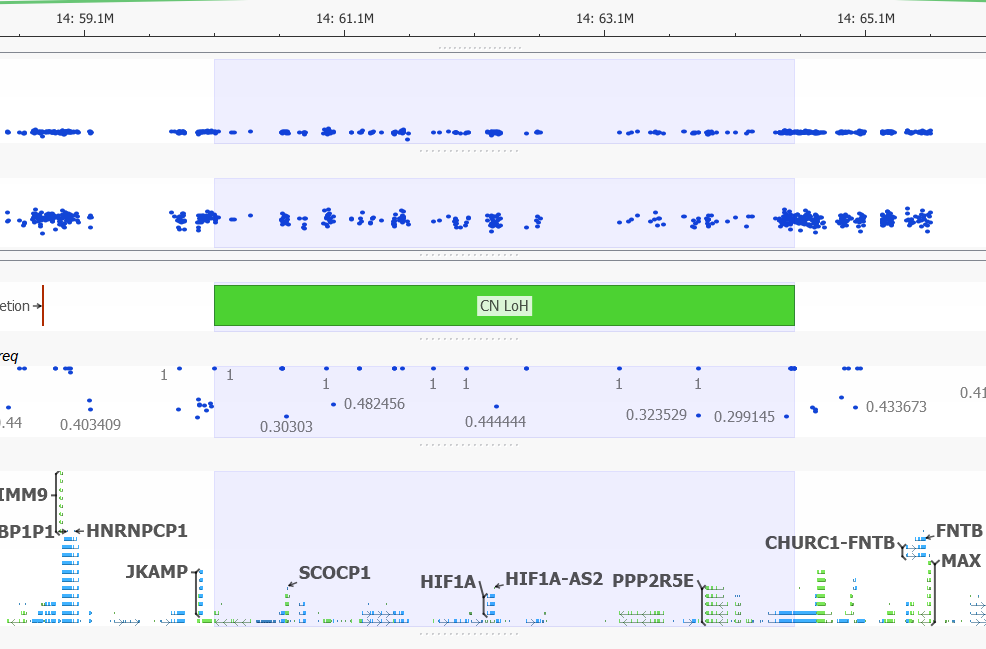
Figure 14. Copy Neutral LOH Event.
Hopefully these frequently asked questions satisfy your curiosity, but if you have additional questions about VarSeq, the Support Team at Golden Helix is happy to answer them! Email us at support@goldenhelix.com.