This is a 2-part series on CNV setup & quality assessment – read part 1 here.

In the final stage of our first blog in this series, the CNV algorithm was run and produced the CNV table. Now the focus will be on filtering to high quality and known CNVs, checking to see if our samples are all high quality, and how to track CNVs across multiple projects using assessment catalogs. Let’s start with some key steps in filtering CNVs.

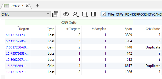
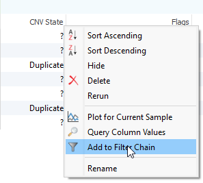
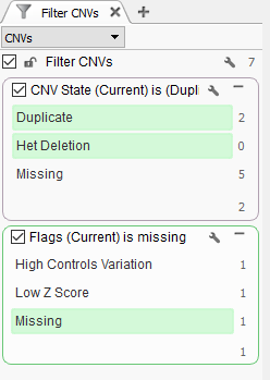
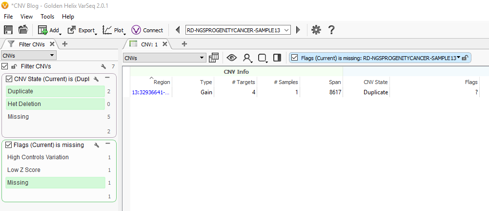
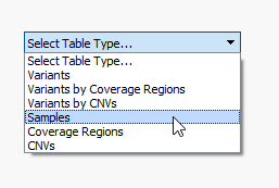
After running the CNV caller, the list of the CNVs in the table reflect all CNVs across all samples. Therefore, some events are listed with a CNV State as missing (?) (Fig 1). Let’s start by filtering to events only seen in one specific sample. Right-click on the CNV State column header and select Add to Filter Chain (Fig 2), and you’ll see the new filter card generate in your CNV filter chain.

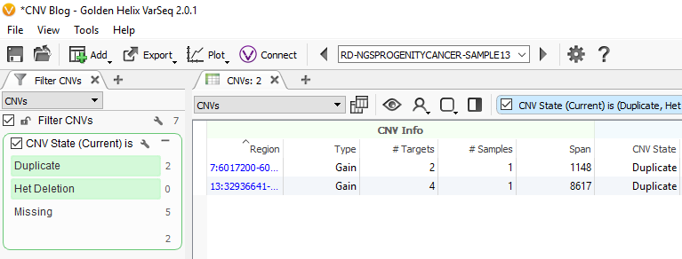
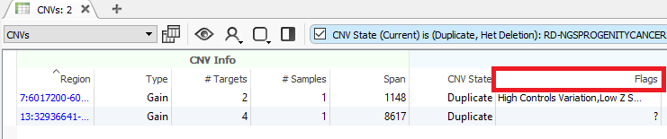
Now we are looking at CNV events specific to Sample 13, and we can start filtering on which events are high quality. To start, let’s filter on the Flag field. When filtering on Flags you’ll want to capture the missing criteria in the filter card (Fig 3a & b). The reason being is that if there is no quality flag (i.e. missing data or ?) then you will capture the high-quality CNVs at the bottom of the filter chain. In Sample 13 we are going to eliminate one event due to it having low-quality flags (Fig 3c)

Here is the list of potential CNV event flags you may encounter:

• Low Controls Depth: Mean read depth over controls exceeded the threshold.
• High Controls Variation: Variation coefficient exceeded the threshold.
• Within Regional IQR: Event is not significantly different from surrounding normal regions based on regional IQR.
• Low Z Score: Event is not significantly different from surrounding normal regions based on regional IQR.

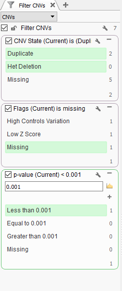
Another quality field we can include in our filter chain is the p-value field. The p-value is the probability that the z-score (standard deviation value of the event) at least as extreme as those in the event would occur by chance. The user can set the confidence threshold to their needs, but you can easily filter down to strong calls by setting a strict confidence value (Fig 4).

Additional quality considerations include looking at the sample level information which can be seen in the samples table (Fig 5a). The samples table is helpful in seeing if there are any low-quality sample flags and also get an idea of how similar the individual SOI (Sample of Interest; i.e. imported samples) is to the reference samples (Fig 5b).

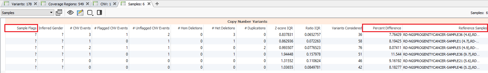
Consider the hypothetical scenario where you have a sample in your project that has a high number of events that don’t seem realistic. The first place you may check is the samples table to see if there are any sample flags and if the percent difference from your reference set is higher than expected. In this project, the maximum percent difference for any sample is about 11.5% which is well below the 20% threshold set with the CNV caller.

Here is the list of potential Sample flags you may encounter:

• High IQR: High interquartile range for Z-score and ratio. This flag indicates that there is high variance between targets for one or more of the evidence metrics.
• High Median Z-score: The median of all the z-scores was above 0.4. This indicates a general skew of this samples away from the reference samples, likely to cause excessive duplication calls.
• Low Sample Mean Depth: Sample mean depth below 30.
• Mismatch to reference samples: Match score indicates low similarity to control samples.
• Mismatch to non-autosomal reference samples: Match score indicates low similarity to non-autosomal control samples.

The quality check steps previously mentioned are likely to fall into your standard workflow and are powerful tools to isolate good quality events. However, the reality is that each users project may present edge case scenarios. So, if you come across events that present more questions or concerns, please don’t hesitate to contact our support staff to assist with clarification in your results.

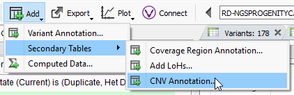
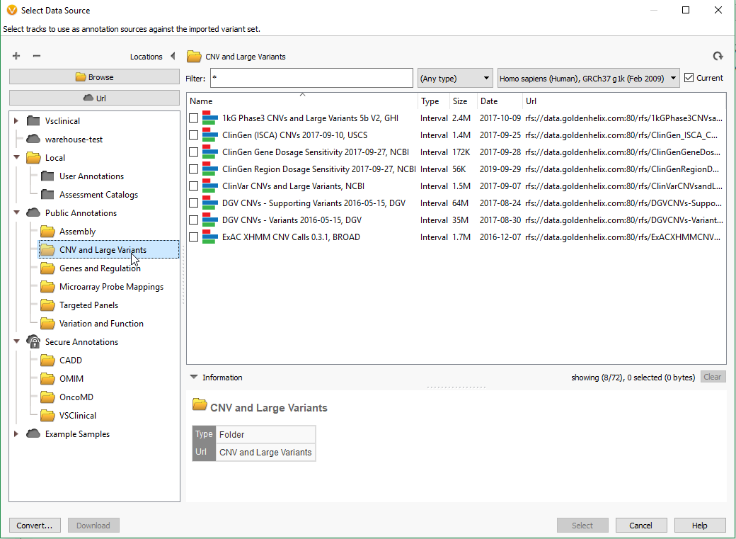
Filtering on quality of events is a great first step in prioritization of your CNV calls, and the next step may be to isolate the obvious events seen in public databases. After you run your CNV caller, you’ll have the option to annotate on the CNV table by clicking on Add -> Secondary Tables -> CNV Annotation (Fig 6a). To gain access to all of the CNV annotations available, click on CNV and large Variants subdirectory under the Public Annotations available on our server.

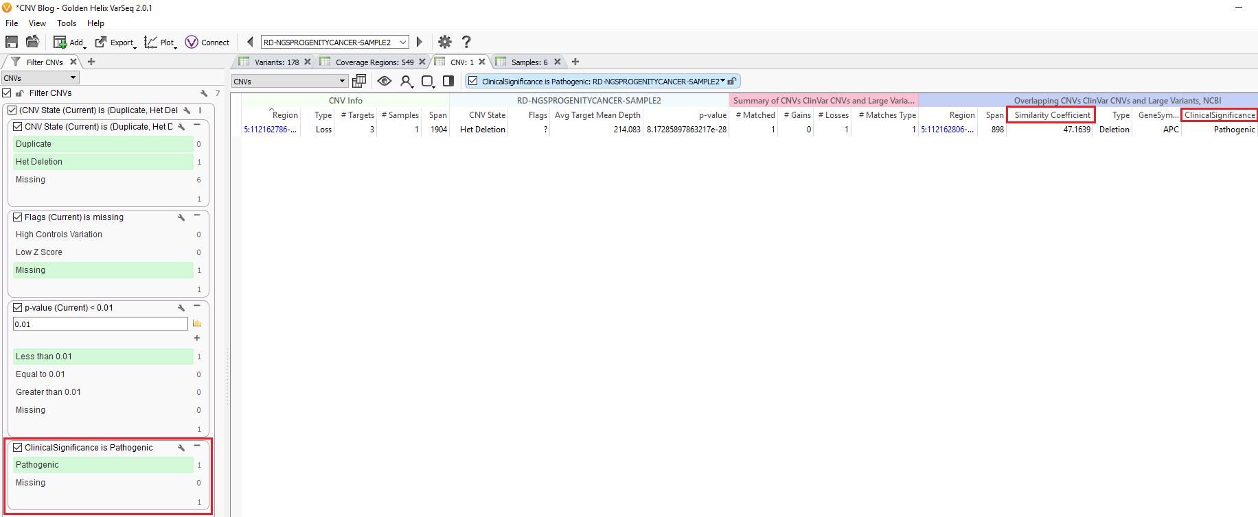
There are numerous annotation tracks to use, and also additional algorithms to explore. Some of these capabilities are presented in recent webcast linked here. Fundamentally, you would want to assess the events you discover that may already be recorded. For example, whether an event is seen as a known pathogenic CNV. This is another field we added to our filter chain and discovered that Sample 2 in our project has a het deletion passing through all the quality filters and recorded in ClinVar as being pathogenic (Fig 7.)

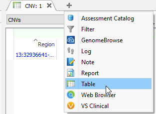
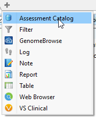
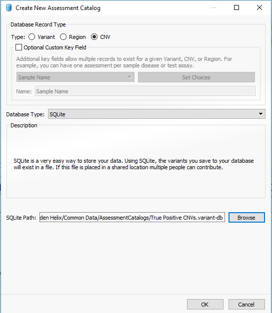
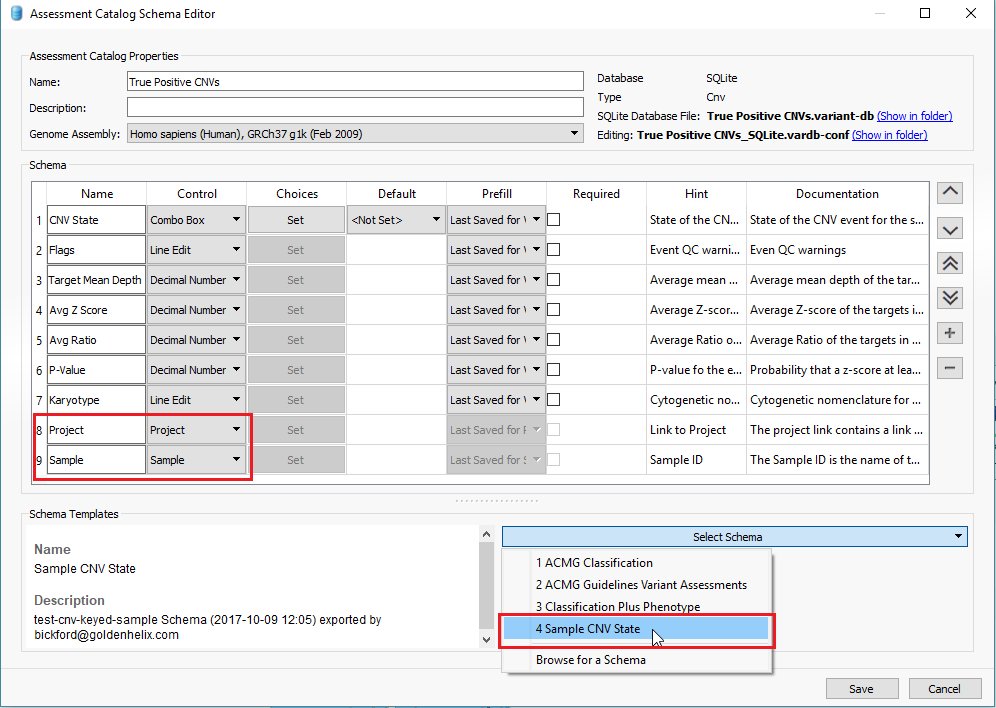
In addition to filtering on curated public annotations, we make available, the user can build their own annotation (i.e. assessment catalog) to track variants/regions/CNVs. Keeping the subject tied to CNVs, the user can easily keep track of events seen across projects. The goal may be to keep track of false or true positive events across samples. In any case, you can build the assessment catalog to keep track of any information you would like. To create a new assessment catalog, click the + icon to open a new tool and select the assessment catalog (Fig 8a). You’ll make the CNV based assessment catalog and decide where you’d like to store the new track being created (Fig 8b). When building the individual fields to be stored in your assessment catalog, you’ll have many customizable options. To simplify this process, we created a schema you can use to build from. In this example, I also added two additional fields: sample and projects records (Fig 8c). Here is a link to the finer details of building an assessment catalog.

In a previous project, I flagged a specific event in Sample 40 and entered all the necessary information for the event in the assessment catalog (Fig 9). All the entered information will be stored in the catalog, and we are going to load it back into the CNV table of our current project. Once you create your assessment catalog, you’ll see it as a list of optional annotations (Fig 9b). When we do this, we see that out of the six SOIs in the project Sample 1 has the same event. This event matches the heterozygous deletion seen in Sample 40 from the previous project (Fig 9c). Users can build assessment catalogs similar to this example to annotate against true events seen in previous samples to confirm true events in future samples.

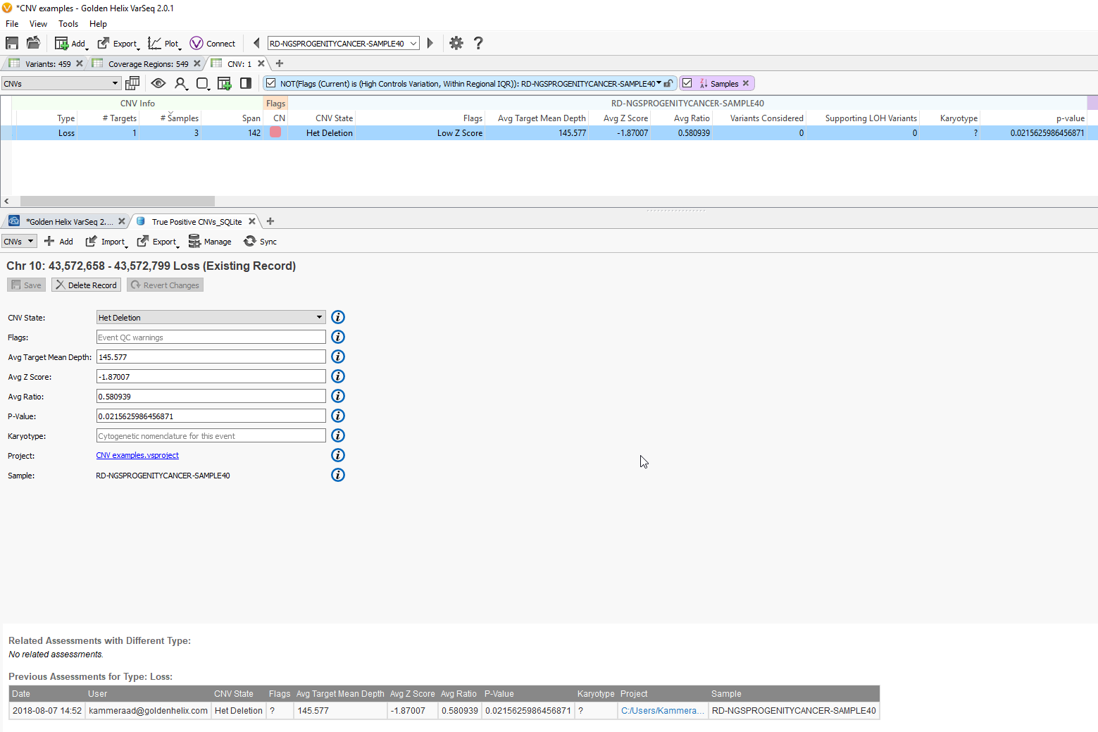
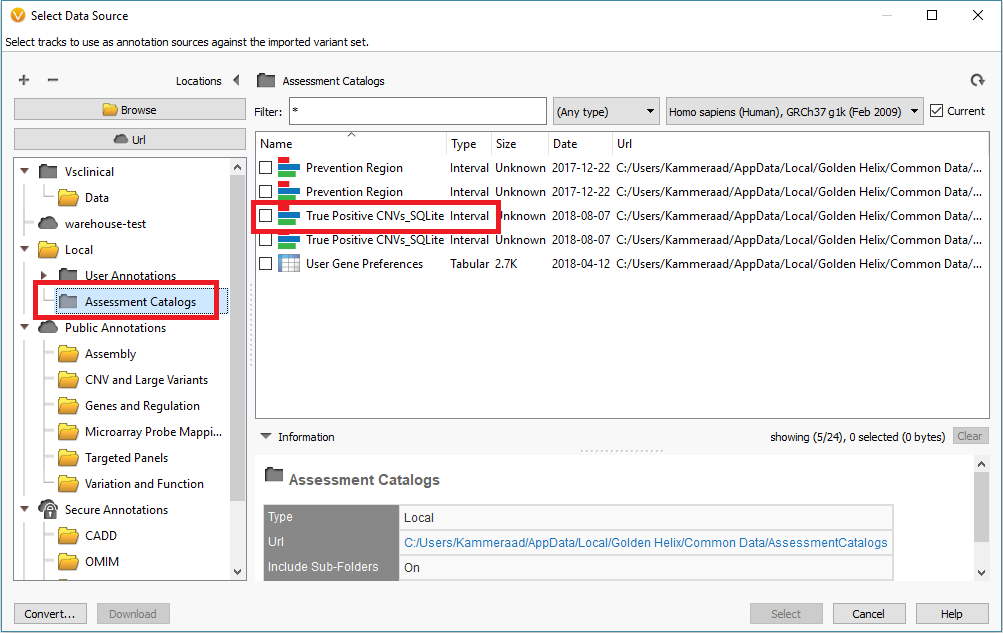
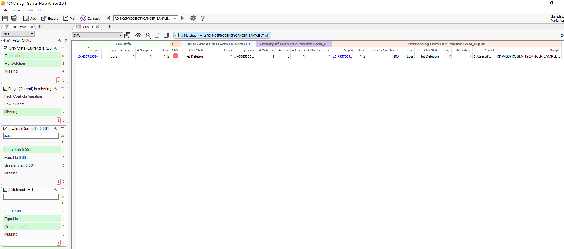
Fig 9c. Adding the assessment catalog to the CNV table allows you to view all the recorded events seen before and that match events in other projects.

With this two-part blog series, users should now be able to perform CNV analysis using their data, set up basic quality filter standards to isolate high-quality events and utilize annotations to hone in on publicly known events as well as in-house recorded CNVs from previous projects. There are a number of features to explore with CNVs and other tools in VarSeq and we would strongly recommend you reach out to us at Golden Helix support (support@goldenhelix.com) if you have any questions on capabilities.

Looking for genetic analysis software to call CNVs? Start a free trial with Golden Helix today.